7 n-step Bootstrapping
- n-step methods generalize both MC methods and one-step TD methods so that one can shift from one to the other smoothly as needed to meet the demands of a particular task.
- n-step methods span a spectrum with MC methods at one end and one-step TD methods at the other.
- The best methods are often intermediate between the 2 extremes.
- n-step methods enable bootstrapping to occur over multiple steps, freeing us from the tyranny of the single time step.
- The idea of n-step methods is used as an introduction to the algorithmic idea of eligibility traces, which enable bootstrapping over multiple time intervals simultaneously.
7.1 n-step TD Prediction, \text{TD}(\lambda)
- Let the TD target look n steps into the future.
- Consider estimating V_\pi from sample episodes generated using \pi:
- MC methods perform an update for each visited state based on the entire sequence of observed rewards from that state until the end of the episode.
- One-step TD methods update is based on the one next reward only.
- \mathbf{n}-step: somewhere in between that performs an update based on an intermediate number of rewards (more than 1 but less than all the rewards in the entire episode).
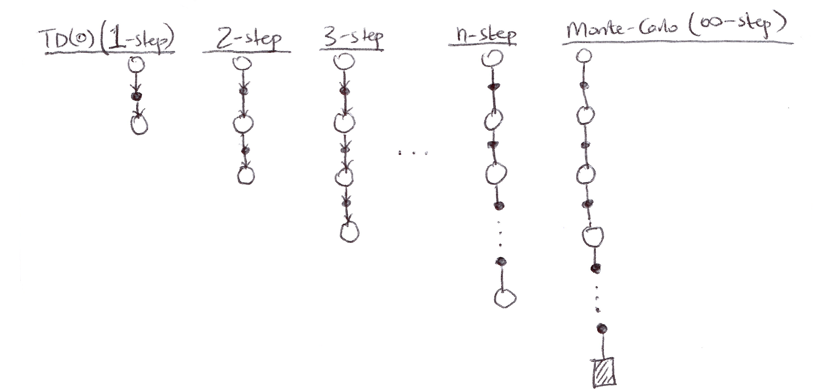
n-step methods are methods in which the temporal difference extends over n steps.
The n-step return looks like:
\begin{aligned} G_t^{(n)} &= G_{t:t+n} \equiv \text{the return from time step } t \text{ to } t+n \\[10pt] n=1\ (\text{TD(0)}): \quad G_t^{(1)} &= R_{t+1} + \gamma V_t(S_{t+1}) \\[6pt] n=2: \quad G_t^{(2)} &= R_{t+1} + \gamma R_{t+2} + \gamma^2 V_{t+1}(S_{t+2}) \\[6pt] &\quad \vdots \\[6pt] n=\infty\ (\text{MC}): \quad G_t^{(\infty)} &= R_{t+1} + \gamma R_{t+2} + \ldots + \gamma^{T-1} R_T \end{aligned}
MC target is the return.
TD(0) target is the one-step return, the first reward plus the discounted next state estimated value (V_t: S \to \mathbb{R} is the estimate at time t of v_\pi).
n-step return:
\boxed{G_t^{(n)} = R_{t+1} + \gamma R_{t+2} + \ldots + \gamma^{n-1} R_{t+n} + \gamma^n V_{t+n-1}(S_{t+n}),}
\forall n, t \quad \text{ s.t. } \quad n \geq 1 \text{ and } 0 \leq t \leq T-n
- All n-step returns can be considered approximations to the full return, truncated after n steps and then corrected for the remaining missing terms by V_{t+n-1}(S_{t+n}).
- If the n-step return extends to or beyond termination, then all the missing terms are taken as zero, and the n-step return becomes the ordinary full return:
G_{t:t+n} = G_t^{(n)} \doteq G_t \quad \text{if } t+n \geq T
- n-step returns for n > 1 involve future rewards and states that are not available at the transition time from t \to t+1. Hence the n-step return cannot be used until after it has seen R_{t+n} and computed V_{t+n-1} when they are both available at time t+n.
The natural state-value learning algorithm for using n-step returns is thus:
V_{t+n}(S_t) \doteq V_{t+n-1}(S_t) + \alpha\left[G_t^{(n)} - V_{t+n-1}(S_t)\right], \quad 0 \leq t < T
while the values of all other states remain unchanged:
V_{t+n}(s) = V_{t+n-1}(s), \quad \forall s \neq S_t
This algorithm is the n-step TD:
\boxed{V(S_t) \leftarrow V(S_t) + \alpha\left[G_t^{(n)} - V(S_t)\right]}
- The n-step return uses the value function V_{t+n-1} to correct for the missing rewards beyond R_{t+n}. An important property of n-step returns is that their expectation is guaranteed to be a better estimate of v_\pi than V_{t+n-1} is in a worst-state sense. This is called the error reduction property. Using this property, all n-step TD methods converge to the correct predictions:
\max_s \left|\mathbb{E}_\pi\left[G_t^{(n)} \mid S_t = s\right] - v_\pi(s)\right| \leq \gamma^n \max_s \left|V_{t+n-1}(s) - v_\pi(s)\right|
7.2 n-step Sarsa, \text{Sarsa}(\lambda)
- n-step value function prediction can be extended to control.
- Switch value function updates based on state rewards to state-action value function updates based on state-action pairs and then use an \varepsilon-greedy policy.
- Backup diagrams for n-step Sarsa are similar to those of n-step TD, consisting of strings of alternating states and actions, except that the Sarsa ones all start and end with an action rather than a state.
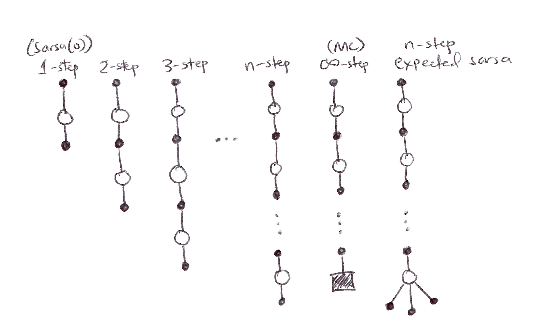
- Consider the following n-step returns for n = 1, 2, \ldots, \infty:
\begin{aligned} G_t^{(n)} &= G_{t:t+n} \\[10pt] n=1\ (\text{Sarsa(0)}): \quad G_t^{(1)} &= R_{t+1} + \gamma Q(S_{t+1}, A_{t+1}) \\[6pt] n=2: \quad G_t^{(2)} &= R_{t+1} + \gamma R_{t+2} + \gamma^2 Q(S_{t+2}, A_{t+2}) \\[6pt] &\quad \vdots \\[6pt] n=\infty\ (\text{MC}): \quad G_t^{(\infty)} &= R_{t+1} + \gamma R_{t+2} + \ldots + \gamma^{T-1} R_T \end{aligned}
- n-step Q-return:
\boxed{G_t^{(n)} \doteq R_{t+1} + \gamma R_{t+2} + \ldots + \gamma^{n-1} R_{t+n} + \gamma^n Q_{t+n-1}(S_t, A_t)}
\forall n, t \quad \text{ s.t. } \quad n \geq 1,\ 0 \leq t \leq T-n, \quad \text{with } G_t^{(n)} = G_t \text{ if } t+n \geq T
- The natural state-action value learning algorithm is then:
Q_{t+n}(S_t, A_t) \doteq Q_{t+n-1}(S_t, A_t) + \alpha\left[G_t^{(n)} - Q_{t+n-1}(S_t, A_t)\right], \quad 0 \leq t < T
Q_{t+n}(s,a) = Q_{t+n-1}(s,a) \quad \forall s, a \quad \text{ s.t. } \quad s \neq S_t \text{ or } a \neq A_t
- This algorithm is called n-step Sarsa:
\boxed{Q_{t+n}(S_t, A_t) \leftarrow Q_{t+n-1}(S_t, A_t) + \alpha\left[G_t^{(n)} - Q_{t+n-1}(S_t, A_t)\right]}
Expected Sarsa
- Similar to n-step Sarsa (linear string of sample actions and states), except that its last element is a branch over all action possibilities weighted by their probability under \pi.
- The n-step return here is:
G_t^{(n)} = R_{t+1} + \gamma R_{t+2} + \ldots + \gamma^{n-1} R_{t+n} + \gamma^n \bar{V}_{t+n-1}(S_{t+n}), \quad t+n < T
\begin{aligned} \text{with } G_t^{(n)} &= G_t \quad \text{if } t+n \geq T \end{aligned}
- \bar{V}_t(s) is the expected approximate value of state s using the estimated action values at time t, under the target policy:
\bar{V}_t(s) \doteq \sum_a \pi(a|s)\, Q_t(s,a), \quad \forall s \in S
- Expected approximate values are essential for action-value methods in RL.
- If s is terminal, then its expected approximate value is defined to be zero: \bar{V}_t(\mathcal{T}) = 0
7.3 n-step Off-policy Learning
- Recall that off-policy learning entails learning the value function for one policy \pi, while following another policy b (behavior policy).
- Often \pi is the greedy policy for the current Q(s,a) estimate (target policy).
- b is a more exploratory policy, perhaps \varepsilon-greedy.
- In order to use the data from b, we must account for the difference between the two policies, using their relative probability of taking the actions that were taken.
- In n-step methods, returns are constructed over n steps, so we are interested in the relative probability of just those n actions.
- For example, to make a simple off-policy n-step TD, we can weight the update for time t (made at time t+n actually) by the importance sampling ratio:
\rho_{t:h} = \prod_{k=t}^{\min(h,\, T-1)} \frac{\pi(A_k|S_k)}{b(A_k|S_k)}
\begin{aligned} \text{where } \rho_{t:h} &\equiv \text{relative probability under the two policies of} \\ &\quad \text{taking the } n \text{ actions from } A_t \text{ to } A_{t+n-1} \end{aligned}
- The off-policy n-step TD update when weighted by \rho_{t:h} becomes:
\boxed{V_{t+n}(S_t) \leftarrow V_{t+n-1}(S_t) + \alpha\, \rho_{t:t+n-1}\left[G_t^{(n)} - V_{t+n-1}(S_t)\right], \quad 0 \leq t < T}
- If both policies are actually the same (on-policy), then the importance sampling ratio is always 1 and we have our previous update (on-policy n-step TD):
\text{if } \pi = b,\ \rho_{t:h} = 1 \implies V(S_t) \leftarrow V(S_t) + \alpha\left[G_t^{(n)} - V(S_t)\right]
Cannot use importance sampling if b = 0 & \pi \neq 0.
Similarly, the n-step Sarsa update can be extended for the off-policy method:
Q_{t+n}(S_t, A_t) \leftarrow Q_{t+n-1}(S_t, A_t) + \alpha\, \rho_{t+1:t+n}\left[G_t^{(n)} - Q_{t+n-1}(S_t, A_t)\right]
- Note that the importance sampling ratio here starts and ends one step later than for n-step TD because we are updating a state-action pair:
- (n-step Sarsa) \rho_{t+1:t+n} vs. \rho_{t:t+n-1} (n-step TD)
- We know that we have selected the action so we need importance sampling only for the subsequent actions.
- For the n-step Expected Sarsa off-policy version, the update is:
\boxed{Q(S_t, A_t) \leftarrow Q(S_t, A_t) + \alpha\, \rho_{t+1:t+n-1}\left[G_t^{(n)} - Q(S_t, A_t)\right]}
- This is the same as the n-step Sarsa update except that the importance sampling ratio used is \rho_{t+1:t+n-1} instead of \rho_{t+1:t+n}, because in Expected Sarsa all possible actions are taken into account in the last state; the one actually taken has no effect and does not need to be corrected for.
7.4 Per-decision Methods with Control Variates
The multi-step off-policy methods presented in section 7.3 are simple and conceptually clear but not very efficient and dramatically increase variance.
A more sophisticated approach would be using per-decision importance sampling.
The ordinary n-step return can be written recursively. For the n-steps ending at horizon h, the n-step return can be written:
G_{t:h} = R_{t+1} + \gamma G_{t+1:h}, \quad t < h < T
\begin{aligned}\text{where } G_{h:h} &\doteq V_{h-1}(S_h)\end{aligned}
Consider the effect of following a behavior policy b that is not the same as the target policy \pi. All of the resulting experiences, including the first reward R_{t+1} and the next state S_{t+1}, must be weighted by the importance sampling ratio for time t:
\rho_t = \frac{\pi(A_t \vert S_t)}{b(A_t \vert S_t)}
A simple approach would be to weight the RHS (R_{t+1} + \gamma G_{t+1:h}) by \rho_t, but a more sophisticated approach would be to use an off-policy definition of the n-step return ending at horizon h:
\boxed{\begin{aligned} G_{t:h} &\doteq \rho_t\left(R_{t+1} + \gamma G_{t+1:h}\right) + (1 - \rho_t) V_{h-1}(S_t), \quad t < h < T \\[6pt] G_{h:h} &\doteq V_{h-1}(S_h) \end{aligned}}
If \rho_t = 0 (trajectory has no chance of occurrence under the target policy), then instead of the target G_{t:h} being zero and causing the estimate to shrink, the target is the same as the estimate and causes no change.
The additional term (1 - \rho_t) V_{h-1}(S_t) is called a control variate and essentially ensures we ignore the sample when the importance sampling ratio is zero, thereby leaving the estimate unchanged.
- The control variate does not change the expected update.
- The importance sampling ratio has an expected value of 1 and is uncorrelated with the estimate, so the expected value of the control variate is zero.
For Action Values
- For action values, the off-policy definition of the n-step return is a little different because the first action does not play a role in the importance sampling (it has already been taken).
- The n-step on-policy return ending at horizon h can be written recursively, and for action values the recursion ends with G_{h:h} \doteq V_{h-1}(S_h). An off-policy form with control variates is:
\boxed{\begin{aligned} G_{t:h} &\doteq R_{t+1} + \gamma\left[\rho_{t+1} G_{t+1:h} + \bar{V}_{h-1}(S_{t+1}) - \rho_{t+1} Q_{h-1}(S_{t+1}, A_{t+1})\right] \\[6pt] &= R_{t+1} + \gamma\, \rho_{t+1}\left(G_{t+1:h} - Q_{h-1}(S_{t+1}, A_{t+1})\right) + \gamma \bar{V}_{h-1}(S_{t+1}), \quad t < h \leq T \end{aligned}}
If h < T, then the recursion ends with G_{h:h} \doteq Q_{h-1}(S_h, A_h).
If h \geq T, the recursion ends with G_{T-1:h} = R_T.
The resultant prediction algorithm (after combining with n-step Sarsa update rule) is analogous to Expected Sarsa.
Importance sampling results in high variance updates. Off-policy training is inevitably slower than on-policy training. Ways to reduce the variance include:
- Control Variates
- Adapt the step size to the observed variance (Autostep Method)
- Invariant updates of Karampatziakis & Langford [2010]
- The usage technique by Mahmood [2017; Mahmood & Sutton, 2015]
7.5 Off-policy Learning Without Importance Sampling: The n-step Tree Backup Algorithm
- Off-policy learning without importance sampling:
- Q-learning & Expected Sarsa do it for the one-step case.
- The n-step case is called the tree-backup algorithm.
- 3-step tree backup diagram:
- 3 sample states & rewards.
- 2 sample actions.
- A list of unselected actions for each state.
- We have no sample for the unselected actions, so therefore we bootstrap using their estimated values.
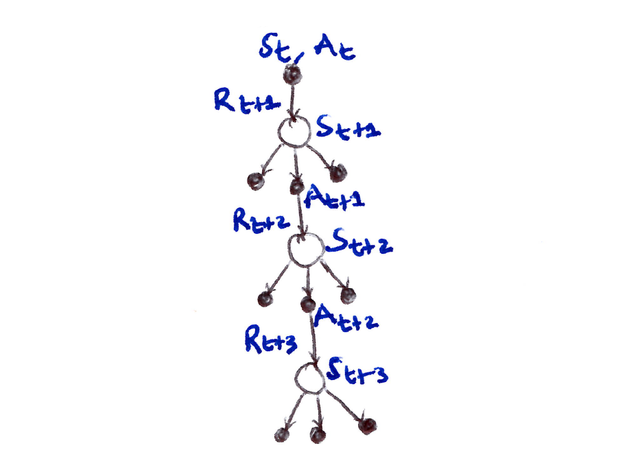
- The target for the update of a node was obtained by combining the rewards along the way and the estimated values of the nodes at the bottom.
- Hence the name, tree-backup update: an update from the entire tree of estimated action values.
- More precisely, the update is from the estimated action values of the leaf nodes of the tree.
- The interior action nodes, corresponding to the actual actions taken, do not participate.
- Each leaf node contributes to the target with a weight proportional to its probability of occurring under the target policy \pi:
- Each first-level action a contributes with a weight of \pi(a|S_{t+1}).
- The action actually taken, A_{t+1}, does not contribute at all and its probability \pi(A_{t+1}|S_{t+1}) is used to weight all the 2nd-level action values.
- Each non-selected 2nd-level action a' contributes with weight \pi(A_{t+1}|S_{t+1})\,\pi(a'|S_{t+2}).
- Each 3rd-level action a'' contributes with weight \pi(A_{t+1}|S_{t+1})\,\pi(A_{t+2}|S_{t+2})\,\pi(a''|S_{t+3}), and so on.
- Essentially each arrow to an action node in the diagram is weighted by the action’s probability of being selected under the target policy and, if there’s a tree below the action, then that weight applies to all leaf nodes in the tree.
Detailed Equations for the n-step Tree-Backup Algorithm
- The one-step return (target) is the same as that of Expected Sarsa:
\begin{aligned} G_{t:t+n} &= G_t^{(n)} \\[6pt] G_t^{(1)} &\doteq R_{t+1} + \gamma \sum_a \pi(a \vert S_{t+1})\, Q_t(S_{t+1}, a), \quad \text{for } t < T-1 \end{aligned}
- The two-step tree-backup return is, for t < T-2:
\begin{aligned} G_t^{(2)} &\doteq R_{t+1} + \gamma \sum_{a \neq A_{t+1}} \pi(a \vert S_{t+1})\, Q_{t+1}(S_{t+1}, a) + \gamma\pi(A_{t+1} \vert S_{t+1})\left(R_{t+2} + \gamma \sum_a \pi(a \vert S_{t+2})\, Q_{t+1}(S_{t+2}, a)\right) \\[6pt] &= R_{t+1} + \gamma \sum_{a \neq A_{t+1}} \pi(a \vert S_{t+1})\, Q_{t+1}(S_{t+1}, a) + \gamma\pi(A_{t+1} \vert S_{t+2})\, G_{t+1:t+2} \end{aligned}
The n-step tree-backup return is, \text{for } t < T-1,\ n \geq 2:
\boxed{G_t^{(n)} \doteq R_{t+1} + \gamma \sum_{a \neq A_{t+1}} \pi(a|S_{t+1})\, Q_{t+n-1}(S_{t+1}, a) + \gamma\pi(A_{t+1}|S_{t+2})\, G_{t+1:t+n}}
- becomes one-step tree-backup return when n=1 and G_{T-1:t+n} = R_T.
We can use G_t^{(n)} in the Q-update from n-step Sarsa, for 0 \leq t < T:
\boxed{Q_{t+n}(S_t, A_t) \leftarrow Q_{t+n-1}(S_t, A_t) + \alpha\left[G_t^{(n)} - Q_{t+n-1}(S_t, A_t)\right]}
- while the values of all other state-action pairs remain unchanged:
Q_{t+n}(s,a) = Q_{t+n-1}(s,a) \quad \forall s, a \quad \text{ s.t. } \quad s \neq S_t \text{ or } a \neq A_t
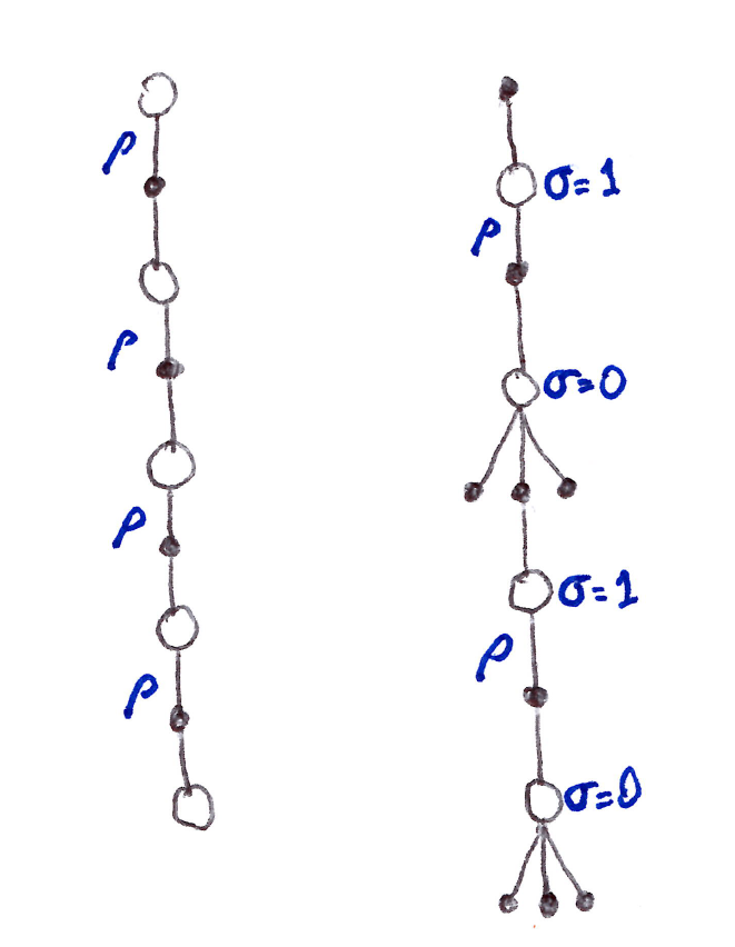
7.6 A Unifying Algorithm: n-step Q(\sigma)
- So far we have considered 3 different kinds of action-value algorithms:
- n-step Sarsa has all sample transitions.
- Tree-backup algorithm has all state-to-action transitions fully branched without sampling.
- n-step Expected Sarsa has all sample transitions except for the last state-to-action one which is fully branched with an expected value.
- Unification Algorithm \Rightarrow One Idea: Decide on a step-by-step basis whether we want to sample, as in Sarsa, or consider the expectation over all actions instead, as in tree-backup update.
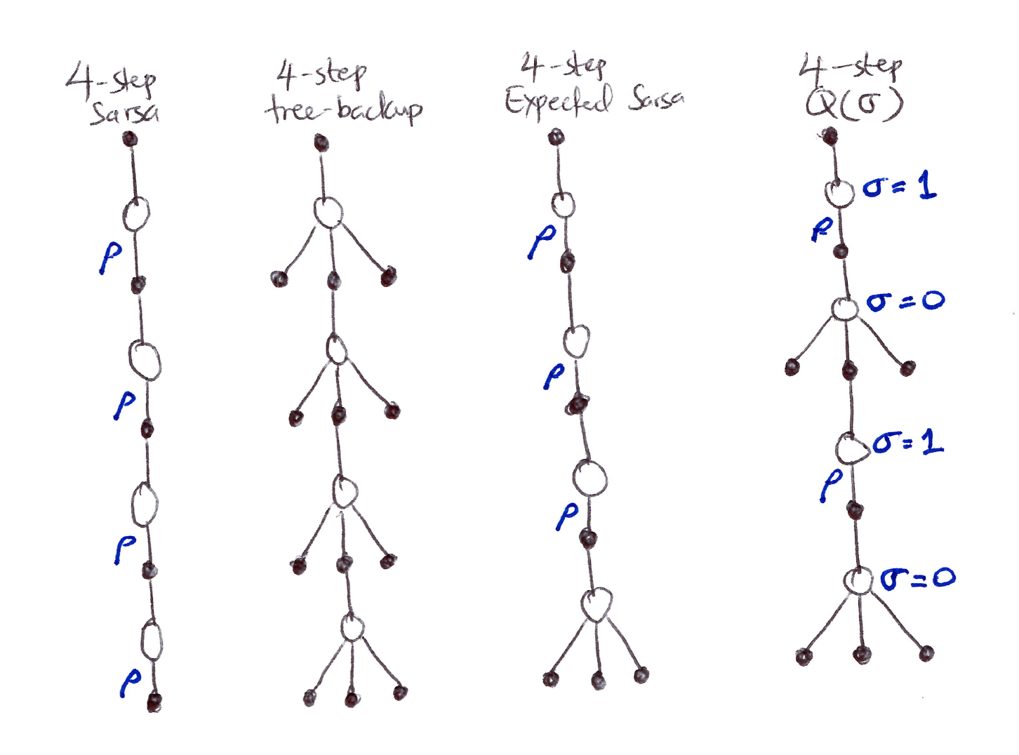
In unification lies many possibilities as seen/suggested in the figure above.
To increase the possibilities even further we can consider a continuous variation between sampling and expectation:
- Let \sigma_t \in [0,1] denote the degree of sampling on step t:
- \sigma = 1 \Rightarrow full sampling
- \sigma = 0 \Rightarrow pure expectation with no sampling
- The random variable \sigma_t might be set as a function of the state, or state-action pair, at time t.
- Let \sigma_t \in [0,1] denote the degree of sampling on step t:
This algorithm is called \mathbf{n}-step \mathbf{Q}(\boldsymbol{\sigma}).
For the equations, first the tree-backup n-step return is expressed in terms of the horizon h = t+n and the expected approximate value \bar{V}:
\begin{aligned} G_{t:h} &= R_{t+1} + \gamma \sum_{a \neq A_{t+1}} \pi(a \vert S_{t+1})\, Q_{h-1}(S_{t+1}, a) + \gamma\pi(A_{t+1} \vert S_{t+1})\, G_{t+1:h} \\[6pt] &= R_{t+1} + \gamma \bar{V}_{h-1}(S_{t+1}) - \gamma\pi(A_{t+1} \vert S_{t+1})\, Q_{h-1}(S_{t+1}, A_{t+1}) + \gamma\pi(A_{t+1} \vert S_{t+1})\, G_{t+1:h} \\[6pt] &= R_{t+1} + \gamma\pi(A_{t+1} \vert S_{t+1})\left[G_{t+1:h} - Q_{h-1}(S_{t+1}, A_{t+1})\right] + \gamma \bar{V}_{h-1}(S_{t+1}) \end{aligned}
- After which it is exactly like the n-step return for Sarsa with control variates except with the action probability \pi(A_{t+1}|S_{t+1}) substituted for the importance sampling ratio \rho_{t+1}. For Q(\sigma), we slide linearly between these 2 cases, \forall\, t < h \leq T:
\boxed{G_{t:h} \doteq R_{t+1} + \gamma\left(\sigma_{t+1}\rho_{t+1} + (1-\sigma_{t+1})\pi(A_{t+1}|S_{t+1})\right)\left(G_{t+1:h} - Q_{h-1}(S_{t+1}, A_{t+1})\right) + \gamma \bar{V}_{h-1}(S_{t+1})}
- The recursion ends with G_{h:h} = 0 if h < T or G_{T-1:T} = R_T if h = T.
- Now we can plug the new defined return into the n-step Sarsa update w/o importance sampling (handled already in G_{t:h}).
7.7 Summary
- There exist a range of TD learning methods that lie in between the one-step TD (TD(0)) methods and Monte Carlo methods. These are n-step methods.
- These methods involve an intermediate amount of bootstrapping and are important because they will typically perform better than either extreme.
- n-step methods look ahead to the next n rewards, states, and actions.
- The two 4-step backup diagrams below together summarize most of the methods introduced:
- n-step TD with importance sampling
- n-step Q(\sigma) which generalizes Expected Sarsa & Q-learning.
- Limitations of n-step methods:
- n time step delay before updating.
- More computation per time step than previously covered methods.
- Require more memory to record the states, actions, rewards, and sometimes other variables over the last n time steps than the one-step methods.
- In Chapter 12, we’ll learn how multi-step TD methods can be implemented with minimal memory and computational complexity using eligibility traces.
- n-step methods, while being quite complex, are conceptually clear. Hence the development of two n-step off-policy learning approaches based on:
- Importance-sampling: conceptually simple but has high variance.
- Tree-based backup updates: natural extension of Q-learning to the multi-step case with stochastic target policies.