3 Finite Markov Decision Processes
- MDPs are a classical formalization of sequential decision making, where actions influence not just immediate rewards, but also subsequent states, and through those future rewards.
- Hence, there exists a tradeoff between delayed and immediate rewards.
- In bandit problems, we estimated q_{*}(a) of each action a.
- In MDPs, we estimate the value q_{*}(s, a) of each action a in each state s.
- These state-dependent action-values are essential for accurate credit assignment for long-term consequences to individual action selections.
- Markov Decision Processes (MDPs) are a mathematical idealized form of the reinforcement learning problem.
- To build the full reinforcement learning (RL) problem’s mathematical structure, key elements are introduced: returns, value functions, & Bellman equations.
3.1 The Agent-Environment Interface
Agent-Environment loop:
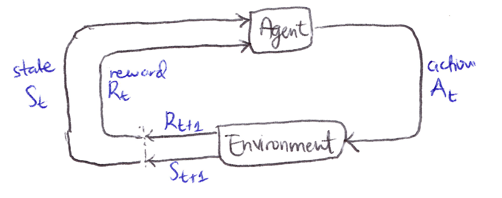
- The agent is the learner and decison maker, while the environment is everything outside the agent that the agent interacts with.
- The agent selects actions, and the environment responds with new states back to the agent.
- The environment also yields rewards, numerical values which the agent seeks to maximize over time through its choice of actions.
- The agent and environment interact continually over a sequence of discrete time steps, t = 0, 1, 2, 3, \dots
- The MDP and agent together yield a recurring sequence of S_t, A_t, R_{t+1}, S_{t+1} or a trajectory when expanded out for all the time steps
\textbf{Trajectory, }\mathcal{T} \equiv (S_0, A_0, R_1, S_1, A_1, R_2, S_2, A_2, R_3, \ldots )
Dynamics function
- In a finite MDP, the sets of states S, actions A, and rewards R are all finite. The random variables S_t and R_t have well-defined discrete probability distributions dependent only on the preceding state and action, this is the Markov property.
- The transition dynamics are fully characterized by the function p, which gives the probability of transitioning to state s' \in S and receiving reward r \in R, given state s and action a
- \forall\ s', s \in \mathcal{S},\, r \in \mathbb{R},\, a \in \mathcal{A}(s), the dynamics function is:
\boxed{p(s', r \mid s, a) \doteq \mathbb{P}\{S_t = s',\, R_t = r \mid S_{t-1} = s,\, A_{t-1} = a\} }
- The dynamics function is an ordinary deterministic function of 4 arguments:
p : \mathcal{S} \times \mathcal{R} \times \mathcal{S} \times \mathcal{A} \to [0,1]
- The “|” in the middle of p(s, r \vert s, a) signifies conditional probability, which reminds us that p specifies a probability distribution for each choice of s and a. i.e., that
\sum_{s' \in \mathcal{S}} \sum_{r \in \mathcal{R}} p(s', r \mid s, a) = 1 \quad \forall\, s \in \mathcal{S},\, a \in \mathcal{A}(s)
Derived quantities
- From the 4-argument dynamics function, p, we can compute anthing we want to know about the environment. Let’s go through some of these functions of interest below.
State-transition/Transition probability function
- State-transition probabilities as a 3-argument function p: S \times S \times A \to [0,1]
p(s'|s,a) \doteq \mathbb{P}\{S_t = s' \mid S_{t-1} = s,\, A_{t-1} = a\} = \sum_{r \in R} p(s', r | s, a)
Reward function for (s,a) pair
- Expected rewards for state-action pairs as a 2-argument function r: S \times A \to \mathbb{R}
r(s,a) \doteq \mathbb{E}\left[R_t \mid S_{t-1} = s,\, A_{t-1} = a\right] = \sum_{r \in R} r \sum_{s' \in S} p(s', r | s, a)
Reward function for (s,a,s') triple
- Expected rewards for state-action-next-state triples as a 3-argument function r: S \times A \times S \to \mathbb{R}
r(s,a,s') \doteq \mathbb{E}\left[R_t \mid S_{t-1} = s,\, A_{t-1} = a,\, S_t = s'\right] = \sum_{r \in R} r\, \frac{p(s', r | s, a)}{p(s' | s, a)}
3.2 Goals & Rewards
- At each time step, the reward is a simple number, R_t \in \mathbb{R}
- The agent’s goal is to maximize the cumulative reward it receives in the long run not the immediate reward.
- This idea was formalized by the reward hypothesis.
All of what we mean by goals and purposes can be well thought of as the maximization of the expected value of the cumulative sum of a received scalar signal (called reward).
- The agent always learns to maximize its reward. If we want it to do something for us, we must provide rewards to it in such a way that in maximizing them the agent will also achieve our goals.
- The reward signal is our way of communicating to the agent what we want it to achieve, not how we want it achieved.
3.3 Returns & Episodes
- The formal definition of the maximization of the cumulative reward received by the agent in the long run leads to the expected return, G_t we want to maximize:
G_t \doteq R_{t+1} + R_{t+2} + R_{t+3} + \ldots + R_T, \quad \quad T = \text{final time step}
- Episodes are finite sequences of interactions between an agent and environment that have a natural terminal state, after which the process resets to a starting state. Each episode is independent, beginning from an initial state and ending at a terminal state S_T.
- An episode is basically a trajectory with a defined endpoint S_T.
\textbf{Episode } \equiv (S_0, A_0, R_1, S_1, A_1, R_2, S_2, A_2, R_3, \ldots, S_T )
- Episodic tasks: Tasks with episodes that have a terminal state, S_T
- Continuing tasks: Tasks with no terminal state (T_{\text{final}} = \infty)
Discounting
- \gamma \equiv discount rate/factor
- \gamma \Rightarrow determines the present value of future rewards
- 0 \leq \gamma \leq 1
- \gamma \approx 0 : “myopic” agent
- \gamma \to 1 : “far-sighted” agent
\boxed{G_t \doteq R_{t+1} + \gamma R_{t+2} + \gamma^2 R_{t+3} + \ldots = \sum_{k=0}^{\infty} \gamma^k R_{t+k+1}}
Recursive form of Expected return
\begin{align*} G_t &= R_{t+1} + \gamma R_{t+2} + \gamma^2 R_{t+3} + \gamma^3 R_{t+4} + \ldots \\ &= R_{t+1} + \gamma\left(R_{t+2} + \gamma R_{t+3} + \gamma^2 R_{t+4} + \ldots\right) \\ &= R_{t+1} + \gamma G_{t+1} \end{align*}
- From G_t = \sum_{k=0}^{\infty} \gamma^k R_{t+k+1}, the expected return is finite if R \neq 0 \text{ and constant, if } \gamma < 1. For example, if R = \text{a constant } + 1 at each timestep, then the discounted return is:
G_t = \sum_{k=0}^{\infty} \gamma^k = \frac{1}{1-\gamma}
3.4 Unified Notation for Episodic & Continuing Tasks
- We can unify the notations for expected return for episodic and continuing tasks into a single notation by considering episode termination to be the entering of a special absorbing state that transitions only to itself and that generates only rewards of 0. For example, lets consider the state transtion diagram:
State transition diagram
S_0 \xrightarrow{R_1=+1} S_1 \xrightarrow{R_2=+1} S_2 \xrightarrow{R_3=+1} \square \circlearrowright \quad \left\{ \begin{array}{l} R_4 = 0 \\ R_5 = 0 \\ \vdots \end{array} \right\}
- The square signifies the special absorbing state that corresponds to the end of an episode.
- Starting from S_0, the reward sequence is +1, +1, +1, 0, 0, 0, \ldots, which when summed yields the same return whether over the first T rewards (T = 3) or over the full infinite sequence, even with discounting present.
- The unified notation, including the possibility that T = \infty or \gamma = 1 (but not both), for the return is:
\boxed{\tilde{G}_t = \sum_{k=t+1}^{T} \gamma^{k-t-1} R_k}
3.5 Policies, Value Functions & Bellman Equations
- Value functions are defined w.r.t. particular ways of acting, called policies.
- A Policy is a mapping from states to probabilities of selecting each possible action.
\boxed{\pi(a|s) = \mathbb{P}\left[A_t = a \mid S_t = s\right]}
- “|” in the middle of \pi(a|s) \Rightarrow reminds us that it defines a probability distribution over a \in A(s) for each s \in S.
- RL methods specify how the agent’s policy is changed as a result of its experience.
State-value function for policy \pi
v_\pi(s) \doteq \mathbb{E}_\pi\left[G_t \mid S_t = s\right] = \mathbb{E}_\pi\left[\sum_{k=0}^{\infty} \gamma^k R_{t+k+1} \,\middle|\, S_t = s\right], \quad \forall s \in S
Action-value function for policy \pi
q_\pi(s,a) \doteq \mathbb{E}_\pi\left[G_t \mid S_t = s,\, A_t = a\right] = \mathbb{E}_\pi\left[\sum_{k=0}^{\infty} \gamma^k R_{t+k+1} \,\middle|\, S_t = s,\, A_t = a\right]
- \mathbb{E}_\pi[\cdot] \Rightarrow expected value of a random variable given that the agent follows policy \pi, if t is any time step.
Bellman Equation for v_\pi
- Recursive self-consistency conditions that must be satisfied by value functions for any policy and state in reinforcement learning and dynamic programming (DP) are called Bellman equations.
\begin{align*} v_\pi(s) &\doteq \mathbb{E}_\pi\left[G_t \mid S_t = s\right] \\ &= \mathbb{E}_\pi\left[R_{t+1} + \gamma G_{t+1} \mid S_t = s\right] \\ &= \sum_a \pi(a \vert s) \sum_{s'} \sum_r p(s', r \vert s, a)\left[r + \gamma\, \mathbb{E}_\pi\left[G_{t+1} \mid S_{t+1} = s'\right]\right] \\ &= \sum_a \pi(a \vert s) \sum_{s', r} p(s', r \vert s, a)\left[r + \gamma v_\pi(s')\right], \quad \forall\, s \in S \end{align*}
This is the Bellman Equation for v_\pi. It expresses the relationship between the value of a state and the value of its successor states.
The Bellman equation averages over all possibilities, weighting each by its probability of occurring.
It states that the starting state value must equal the (discounted) value of the expected next state, plus the reward expected along the way.
We visualize this relationship between a state and its possible successor states with a backup diagram.
It is called a backup diagram because it looks at how value is transferred back up the tree from the possible successor states of a specific state at the bottom of the tree to that specific state at the top of the tree.
Backup Diagrams for v_{\pi}(s)
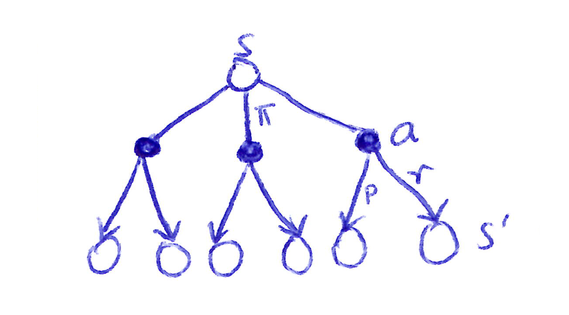
Backup diagram for v_\pi: Each open circle represents a state s, filled circles represent state-action pairs (s, a), next open circles set represent successor states s'.
- A state-value is an expectation over the available action-values under a policy:
\begin{equation} \begin{split} v_{\pi}(s) & \doteq \mathbb{E}_{\pi,p} [G_t\ |\ S_t{=}s]\\ & = \mathbb{E}_{\pi,p} [q_{\pi}(s,A_t)\ |\ S_t{=}s], \quad \text{(cf. [*])}\\ & = \displaystyle \sum_{a} \pi(a|s) q_{\pi}(s,a)\\ \end{split} \end{equation}
[*] Given a state-action pair, the return G_t is an action-value.
G_t is a function of the state s (given by the condition “S_t{=}s”) and the action A_t (given by the policy \pi under the expectation \mathbb{E}_{\pi,p}).
The following recursive relationship satisfied by v_{\pi}(s) is called the Bellman equation for state-values. The value function v_{\pi}(s) is the unique solution to its Bellman equation.
\begin{align*} v_{\pi}(s) & \doteq \mathbb{E}_{\pi,p} [G_t\ |\ S_t{=}s]\\ & = \mathbb{E}_{\pi,p} [R_{t+1} + \gamma G_{t+1}\ |\ S_t{=}s]\\ & = \displaystyle \sum_{a} \pi(a|s) \mathbb{E}_{p,\pi} [R_{t+1} + \gamma G_{t+1}\ |\ S_t{=}s, A_t{=}a ]\\ & = \displaystyle \sum_{a} \pi(a|s) \sum_{s',r} p(s',r|s,a) \mathbb{E}_{\pi,p} [r + \gamma G_{t+1}\ |\ S_t{=}s, A_t{=}a, S_{t+1}{=}s' ]\\ & = \displaystyle \sum_{a} \pi(a|s) \sum_{s',r} p(s',r|s,a) \mathbb{E}_{\pi,p} [r + \gamma G_{t+1}\ |\ S_{t+1}{=}s' ] \;\; \text{(by the Markov property)}\\ & = \displaystyle \sum_{a} \pi(a|s) \sum_{s',r} p(s',r|s,a) \Big[r + \gamma \mathbb{E}_{\pi,p} [G_{t+1}\ |\ S_{t+1}{=}s'] \Big]\\ & = \displaystyle \sum_{a} \pi(a|s) \sum_{s',r} p(s',r|s,a) \Big[r + \gamma v_{\pi}(s') \Big]\\ \end{align*}
- Final form:
\boxed{\begin{array}{rcl} v_{\pi}(s) &=& \displaystyle\sum_{a} \pi(a \vert s)\, q_{\pi}(s,a)\\[1em] &=& \displaystyle\sum_{a} \pi(a \vert s) \sum_{s',r} p(s',r \vert s,a) \Big[r + \gamma v_{\pi}(s') \Big] \end{array}}
Bellman equation for q_{\pi}(s,a)
- An action-value is an expectation over the possible next state-values under the environment’s dynamics.
\begin{align*} q_{\pi}(s,a) & \doteq \mathbb{E}_{p,\pi} [G_t\ |\ S_t{=}s, A_t{=}a]\\ & = \mathbb{E}_{p,\pi} [R_{t+1} + \gamma G_{t+1}\ |\ S_t{=}s, A_t{=}a]\\ & = \mathbb{E}_{p,\pi} [R_{t+1} + \gamma v_{\pi}(S_{t+1})\ |\ S_t{=}s, A_t{=}a], \quad \text{(cf. [*])}\\ & = \displaystyle \sum_{s',r} p(s',r|s,a) \Big[r + \gamma v_{\pi}(s')\Big]\\ \end{align*}
[*] Given only a state s, the return G_t is a state-value.
G_t is a function of the state S_{t+1} (given by the environment’s dynamics p under the expectation \mathbb{E}_{p,\pi}).
The following recursive relationship satisfied by q_{\pi}(s,a) is called the Bellman equation for action-values. The value function q_{\pi}(s,a) is the unique solution to its Bellman equation.
\begin{align*} q_{\pi}(s,a) & \doteq \mathbb{E}_{p,\pi} [G_t\ |\ S_t{=}s, A_t{=}a]\\ & = \mathbb{E}_{p,\pi} [R_{t+1} + \gamma G_{t+1}\ |\ S_t{=}s, A_t{=}a]\\ & = \displaystyle \sum_{s',r} p(s',r|s,a) \mathbb{E}_{\pi,p} [r + \gamma G_{t+1}\ |\ S_t{=}s, A_t{=}a, S_{t+1}{=}s' ]\\ & = \displaystyle \sum_{s',r} p(s',r|s,a) \mathbb{E}_{\pi,p} [r + \gamma G_{t+1}\ |\ S_{t+1}{=}s' ], \quad \text{(by the Markov property)}\\ & = \displaystyle \sum_{s',r} p(s',r|s,a) \Big[r + \gamma \mathbb{E}_{\pi,p} [G_{t+1}\ |\ S_{t+1}{=}s'] \Big]\\ & = \displaystyle \sum_{s',r} p(s',r|s,a) \Big[r + \gamma \sum_{a'} \pi(a'|s') \mathbb{E}_{p,\pi} [G_{t+1}\ |\ S_{t+1}{=}s', A_{t+1}{=}a'] \Big]\\ & = \displaystyle \sum_{s',r} p(s',r|s,a) \Big[r + \gamma \sum_{a'} \pi(a'|s') q_{\pi}(s',a') \Big]\\ \end{align*}
- Final form:
\boxed{\begin{array}{rcl} q_{\pi}(s,a) &=& \displaystyle\sum_{s',r} p(s',r \vert s,a) \Big[r + \gamma v_{\pi}(s')\Big]\\[1em] &=& \displaystyle\sum_{s',r} p(s',r \vert s,a) \Big[r + \gamma \sum_{a'} \pi(a' \vert s')\, q_{\pi}(s',a') \Big] \end{array}}
3.6 Optimal Policies & Optimal Value Functions
- For finite MDPS, we can define an optimal policy for finite MDPs as a policy that achieves the maximum expected return.Value functions define a partial ordering over policies. A policy \pi is better than or equal to \pi' iff v_\pi(s) \geq v_{\pi'}(s) for all s \in S.
\pi \geq \pi' \iff v_\pi(s) \geq v_{\pi'}(s) \quad \forall s \in S
- There always exists at least one optimal policy \pi_{*}, which is better than or equal to all other policies. All optimal policies share the same optimal state-value function v_{*}, defined as:
v_*(s) \doteq \max_\pi v_\pi(s) \quad \forall s \in S
- All optimal policies also share the same optimal action-value function q_{*}, defined as:
q_*(s,a) \doteq \max_\pi q_\pi(s,a) \quad \forall s \in S,\, a \in A(s)
- For a state-action pair (s, a), q_{*} gives the expected return for taking action a in state s and thereafter following an optimal policy. We can therefore write q_{*} in terms of v_{*} as:
q_*(s,a) = \mathbb{E}\left[R_{t+1} + \gamma v_*(S_{t+1}) \mid S_t = s,\, A_t = a\right]
Bellman Optimality Equations
- Self-consistency condition given by Bellman equation for state values must be satisfied by v_{*} and q_{*}.
Optimal state-value function, v_{*}(s)
\begin{align*} v_{*}(s) &= \max_{a \in A(s)} q_{\pi_{*}}(s,a) \\ &= \max_a\, \mathbb{E}_{\pi^*}\left[G_t \mid S_t = s,\, A_t = a\right] \\ &= \max_a\, \mathbb{E}_{\pi^*}\left[R_{t+1} + \gamma G_{t+1} \mid S_t = s,\, A_t = a\right] \\ &= \max_a\, \mathbb{E}\left[R_{t+1} + \gamma v_{*}(S_{t+1}) \mid S_t = s,\, A_t = a\right] \\ &= \max_a \sum_{s', r} p(s', r \vert s, a)\left[r + \gamma v_{*}(s')\right] \end{align*}
\boxed{\begin{array}{rcl} v_{*}(s) &=& \displaystyle \max_a \sum_{s', r} p(s', r \vert s, a)\left[r + \gamma v_{*}(s')\right] \end{array}}
Optimal action-value function, q_{*}(s,a)
\boxed{ \begin{align*}{rcl} q_{*}(s,a) &= \mathbb{E}\left[R_{t+1} + \gamma \max_{a'} q_{*}(S_{t+1}, a') \mid S_t = s,\, A_t = a\right] \\ &= \sum_{s', r} p(s', r \vert s, a)\left[r + \gamma \max_{a'} q_{*}(s', a')\right] \end{align*} }
Backup Diagrams for v_{*}(s) & q_{*}(s,a)
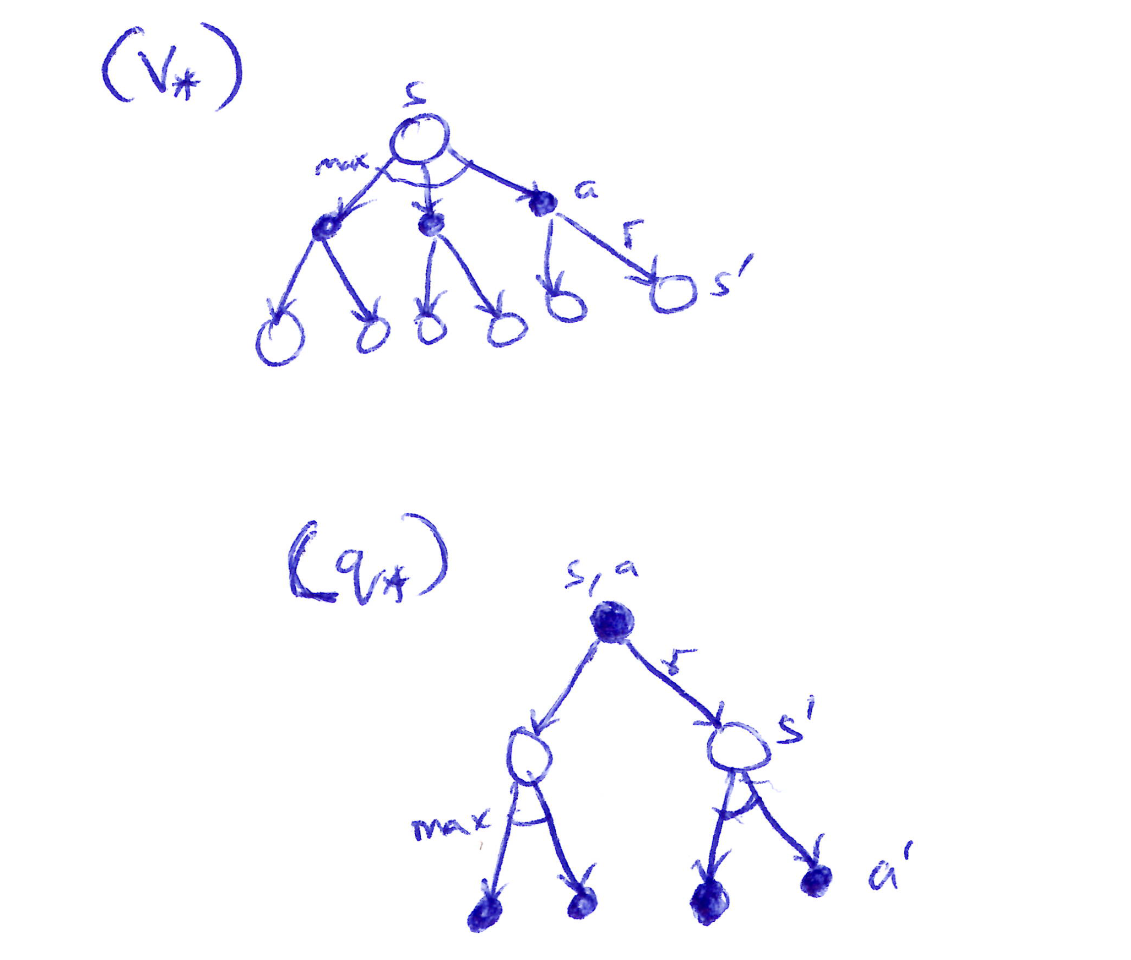
Backup diagrams for v_* and q_*: the max node appears at the state level for v_* and at the successor state level for q_*.
Takeaways
- For finite MDPs, the Bellman optimality equation has a unique solution, a system of n equations in n unknowns (one per state) solvable if the dynamics p are known.
- Any policy that is greedy with respect to v_{*} is an optimal policy: since v_{*} already accounts for all future rewards, a one-step-ahead search is sufficient to identify optimal actions.
- q_{*} makes optimal action selection even easier; the agent simply picks \arg\max_a\, q_{*}(s, a) without needing to know the environment’s dynamics or successor state values.
- Explicitly solving the Bellman optimality equation is rarely practical. It requires 3 assumptions that rarely all hold simultaneously:
- Known environment dynamics,
- Sufficient computational resources, and
- The Markov property
- In practice, RL methods settle for approximate solutions to the Bellman optimality equation, using actual experienced transitions in place of full knowledge of expected transitions.
3.7 Optimality & Approximation
- We have defined optimal value functions and optimal policies clearly.
- A Q-table is not practical/possible in large state spaces.
- Hence, the need for function approximation because calculation of optimality (Q-table) is too expensive.
- Computing optimal policies is rarely feasible in practice due to extreme computational cost, even with a complete and accurate model of the environment’s dynamics.
- The agent is always constrained by available computational power (per time step) and memory, both of which limit how well value functions, policies, and models can be approximated.
- When the state space is small and finite, exact tabular methods suffice; for larger state spaces, function approximation with compact parameterized representations is necessary.
- RL’s online nature allows approximations to focus more effort on frequently encountered states, at the expense of rarely visited ones. This makes useful approximate solutions achievable even when optimal ones are not.
- This ability to prioritize learning for high-frequency states is a key property that distinguishes RL from other approaches to approximately solving MDPs.
3.8 Summary
- RL is about learning from interaction to maximize cumulative reward over time, with the agent-environment interface defined by actions, states, and rewards.
- A finite MDP formalizes this with well-defined transition probabilities over finite state, action, and reward sets.
- The return is the (expected) function of future rewards the agent seeks to maximize (undiscounted for episodic tasks, discounted for tabular continuing tasks).
- Value functions assign expected returns to states or state-action pairs; optimal value functions give the maximum achievable return, and any policy greedy w.r.t. them is optimal.
- Problems vary by knowledge level: complete knowledge gives the agent full dynamics p; incomplete knowledge does not.
- In practice, optimal solutions are rarely computable, therefore memory and computation constraints force agents to approximate value functions, policies, and models.
3.9 Glossary
- Reinforcement Learning: learning from interaction how to behave in order to achieve a goal
- Agent: known & controllable; the RL agent & its environment interact over a sequence of discrete time steps
- Environment: incompletely controllable & may/may not be completely known
- Actions: choices made by the agent
- States: the basis/foundation for making the choices/actions
- Rewards: the basis for evaluating the choices/actions
- Policy: a stochastic rule by which the agent selects actions as a function of states (agent’s brain) \boxed{\pi(a|s) = \mathbb{P}[A_t = a | S_t = s]}
- MDP: the variables formulated above within a RL setup with well-defined transition probabilities
- A finite MDP: an MDP with finite state, action & reward sets.
- MRP: Markov Reward Process
| Markov Property | Markov Chain/Process | MRP | MDP |
|---|---|---|---|
| \mathbb{P}[S_{t+1} \mid S_t] = \mathbb{P}[S_{t+1} \mid S_1, \ldots, S_t] |
\langle S, P \rangle | \langle S, P, R, \gamma \rangle | \langle S, A, P, R, \gamma \rangle |
| State-transition probability matrix: P_{ss'} = \mathbb{P}[S_{t+1} = s' \mid S_t = s] |
Sequences of random states (S_1, S_2, \ldots) + Markov property |
Markov Chain with Values | MRP + decisions |
- MDP components:
\text{MDP} \left\{ \begin{array}{lll} S & \to & \text{finite set of states} \\ A & \to & \text{finite set of actions} \\ P & \to & \text{state transition probability matrix,} \quad P^a_{ss'} = \mathbb{P}[S_{t+1} = s' \vert S_t = s,\, A_t = a] \\ R & \to & \text{reward function,} \qquad\qquad\qquad\qquad\quad R^a_s = \mathbb{E}[R_{t+1} \vert S_t = s,\, A_t = a] \\ \gamma & \to & \text{discount factor,} \qquad\qquad\qquad\qquad\qquad \gamma \in [0,1] \end{array} \right\}
Return: function of future rewards that the agent seeks to maximize (in expected value)
Tasks:
- Episodic: have a clear starting & ending point (a terminal state) [e.g. ping pong]
- Continuing: tasks/RL instances that continue forever w/o a terminal state [e.g. automated stock trading]
Discount factor, \gamma: determines the present value of future rewards
Value functions (v_\pi, q_\pi): a policy’s value functions assign to each state/state-action pair, the expected return from that state/state-action pair, given that the agent uses the policy.
Optimal value functions (v_*, q_*): assign to each state/state-action pair the largest expected return achievable by any policy.
Optimal policy (\pi_*): a policy whose value functions are optimal \left[v_*(s) = \max_\pi v_\pi(s)\right]
- \pi_* > \pi,\ \forall \pi (\pi \geq \pi' iff v_\pi(s) \geq v_{\pi'}(s)\ \forall s \in S)
- v_* & q_* are unique for a given MDP, but there can be many optimal policies (\pi_*)
- Any policy that is greedy w.r.t. the optimal value functions (q_*, v_*) must be an optimal policy (\pi_*)
Bellman Optimality Equations: special consistency conditions that q_*, v_* must satisfy & that can, in principle, be solved for q_*, v_*, from which an optimal policy (\pi_*) can be determined with relative ease.