6 Temporal-Difference Learning
- TD methods learn directly from raw experience.
- TD is model-free (no model of the environment’s dynamics).
- TD methods update estimates based on other learned estimates; in other words TD learns from incomplete episodes. This is called bootstrapping.
6.1 TD Prediction
Goal: Learn/estimate V_\pi from experience under policy \pi.
- Both TD and Monte Carlo (MC) methods use experience to solve the prediction problem.
- A simple incremental every-visit MC suitable for nonstationary environments is:
V(S_t) \leftarrow V(S_t) + \alpha\left[G_t - V(S_t)\right]
\begin{aligned} \text{where } G_t &\equiv \text{actual return following time } t \\[6pt] \alpha &\equiv \text{constant step-size parameter} \end{aligned}
- The simplest TD method, TD(0), makes the update:
\boxed{V(S_t) \leftarrow V(S_t) + \alpha\underbrace{\left[R_{t+1} + \gamma V(S_{t+1}) - V(S_t)\right]}_{\text{TD Error}}}
\begin{aligned} \text{where } R_{t+1} + \gamma V(S_{t+1}) &\equiv \text{the \textbf{TD target}} \end{aligned}
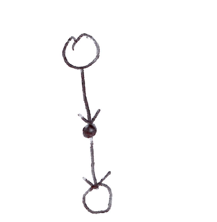
TD(0) backup diagram: one-step lookahead from state s through action to next state s'.
Pseudocode: Tabular TD(0) for Estimating v_\pi
\boxed{ \begin{aligned} &\textbf{Input: } \text{the policy } \pi \text{ to be evaluated} \\ &\textbf{Algorithm parameter: } \text{step size } \alpha \in (0,1] \\ &\textbf{Initialize } V(s) \text{ for all } s \in \mathcal{S}^+\text{, arbitrarily except that } V(\text{terminal}) = 0 \\ &\textbf{Loop for each episode:} \\ &\quad \text{Initialize } S \\ &\quad \textbf{Loop for each step of episode:} \\ &\qquad A \leftarrow \text{action given by } \pi \text{ for } S \\ &\qquad \text{Take action } A\text{, observe } R, S' \\ &\qquad V(S) \leftarrow V(S) + \alpha\!\left[R + \gamma V(S') - V(S)\right] \\ &\qquad S \leftarrow S' \\ &\quad \textbf{Until } S \text{ is terminal} \end{aligned} }
- TD(0) bases its update in part on an existing estimate (bootstrapping):
\begin{align*} v_\pi(s) &\doteq \mathbb{E}\left[G_t \mid S_t = s\right] \\ &= \mathbb{E}_\pi\left[R_{t+1} + \gamma G_{t+1} \mid S_t = s\right] \\ &= \mathbb{E}_\pi\left[R_{t+1} + \gamma v_\pi(S_{t+1}) \mid S_t = s\right] \\ \end{align*}
- The TD target is an estimate because it samples the expected values in the equation above, and it uses the current estimate V instead of the true V_\pi.
- TD methods combine the sampling of MC with the bootstrapping of DP.
TD Error & its Relationship to MC Error
The TD error at each time is the error in the estimate made at that time because the TD error depends on the next state and next reward. If the array V does not change during the episode (like in MC methods), then:
\text{MC error} = \sum_t \text{TD error}
Let \delta_t \doteq R_{t+1} + \gamma V(S_{t+1}) - V(S_t) (the TD error). Then:
\begin{aligned} G_t - V(S_t) &= R_{t+1} + \gamma G_{t+1} - V(S_t) + \gamma V(S_{t+1}) - \gamma V(S_{t+1}) \\[6pt] &= \underbrace{R_{t+1} + \gamma V(S_{t+1}) - V(S_t)}_{\delta_t} + \gamma G_{t+1} - \gamma V(S_{t+1}) \\[6pt] &= \delta_t + \gamma\left(G_{t+1} - V(S_{t+1})\right) \\[6pt] &= \delta_t + \gamma\left(R_{t+2} + \gamma G_{t+2} - V(S_{t+1})\right) \\[6pt] &= \delta_t + \gamma\left(R_{t+2} + \gamma V(S_{t+2}) - V(S_{t+1}) + \gamma G_{t+2} - \gamma V(S_{t+2})\right) \\[6pt] &= \delta_t + \gamma\underbrace{\left(R_{t+2} + \gamma V(S_{t+2}) - V(S_{t+1})\right)}_{\delta_{t+1}} + \gamma^2\left(G_{t+2} - V(S_{t+2})\right) \\[6pt] &= \delta_t + \gamma \delta_{t+1} + \gamma^2\left(G_{t+2} - V(S_{t+2})\right) \\[6pt] &= \delta_t + \gamma \delta_{t+1} + \gamma^2\left(R_{t+3} + \gamma V(S_{t+3}) - V(S_{t+2}) + \gamma G_{t+3} - \gamma V(S_{t+3})\right) \\[6pt] &= \delta_t + \gamma \delta_{t+1} + \gamma^2 \delta_{t+2} + \gamma^3\left(G_{t+3} - V(S_{t+3})\right) \\[6pt] &\quad \vdots \\[6pt] &= \delta_t + \gamma \delta_{t+1} + \gamma^2 \delta_{t+2} + \gamma^3 \delta_{t+3} + \ldots + \gamma^{T-t-1} \delta_{T-1} + \gamma^{T-t}\underbrace{\left[G_T - V(S_T)\right]}_{=\, 0} \end{aligned}
\boxed{G_t - V(S_t) = \sum_{k=t}^{T-1} \gamma^{k-t}\, \delta_k}
6.2 Advantages of TD Prediction Methods
- TD methods are model-free, unlike DP methods.
- TD methods can learn before knowing the final outcome & without the final outcome, unlike MC:
- before: TD can learn online, incrementally, while MC must wait until the episode ends when the return is known.
- without: TD can learn from incomplete sequences/episodes while MC only learns from complete sequences.
- TD works in continuing (non-terminating) environments while MC only works for episodic/terminating environments.
- TD(0) converges to v_\pi(s) for a fixed policy \pi, but not always for general function approximation.
- TD methods are usually more efficient than MC methods (constant \alpha) on stochastic tasks; they converge faster.
- TD methods have low variance, while MC methods have high variance.
6.3 Optimality of TD(0)
- For a finite number of episodes, we can run our methods repeatedly with the same data (finite episodes) until convergence as we continually update the value function by the sum of each of the increments at the end of each batch.
- This is called batch updating because updates are made only after processing each complete batch of training data / finite number of episodes.
- Under batch updating, TD(0) & constant-\alpha MC methods converge deterministically to a single answer independent of \alpha, as long as \alpha is chosen to be sufficiently small.
- In general, batch MC methods always find the estimates that minimize mean square error on the training set, whereas batch TD(0) always finds the estimates that would be exactly correct for the maximum-likelihood model of the Markov process.
- Given this model, we can compute the estimate of the value function that would be exactly correct if the model were exactly correct.
- This is called the certainty-equivalence estimate because it is equivalent to assuming that the estimate of the underlying process was known with certainty rather than being approximated.
- In general, batch TD(0) converges to the certainty-equivalence estimate.
6.4 Sarsa: On-policy TD Control
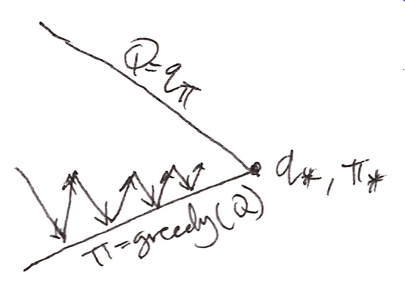
- Using TD prediction methods for control, we’ll follow Generalized Policy Iteration (GPI), only this time using TD methods for the policy evaluation part (predicting the value function).
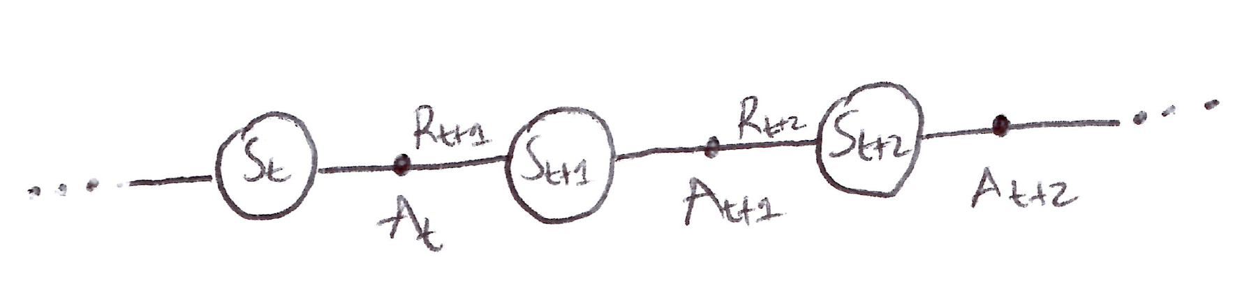
- For on-policy control, we learn an action-value function q_\pi(s,a) for our current policy \pi, for all states s and actions a. Recall that an episode consists of an alternating sequence of states and state–action pairs:
\boxed{Q(S_t, A_t) \leftarrow Q(S_t, A_t) + \alpha\Big[\underbrace{R_{t+1} + \gamma Q(S_{t+1}, A_{t+1})}_{\text{TD target}} - Q(S_t, A_t)\Big]}
- This update rule uses a quintuple of events (S_t, A_t, R_{t+1}, S_{t+1}, A_{t+1}). Hence, the name SARSA. The backup diagram is shown below:
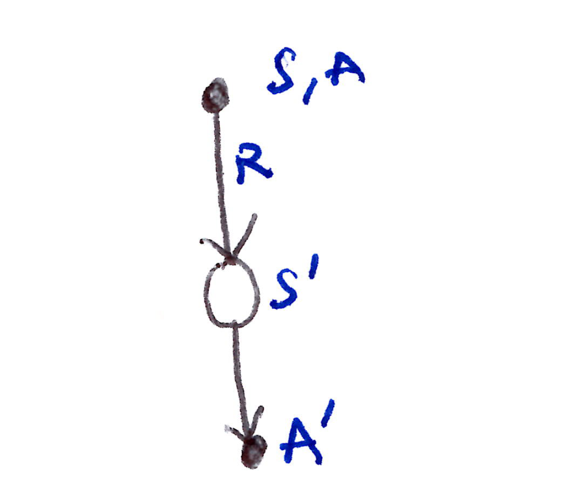
Sarsa backup diagram: from state-action pair (S, A) through reward R to next state S' and next action A'.
As in all on-policy methods, we continually estimate q_\pi for the behavior policy \pi & simultaneously update the policy \pi greedily w.r.t. q_\pi.
The convergence properties of the SARSA algorithm depend on the nature of the policy’s dependence on Q. For example, one could use \varepsilon-greedy / \varepsilon-soft policies.
Goal: Use TD in the control loop
- apply TD to Q(s,a),
- use \varepsilon-greedy policy improvement,
- update with every time-step.
- Every time step:
- Policy Evaluation: SARSA, Q \approx q_\pi
- Policy Improvement: \varepsilon-greedy
Pseudocode: SARSA for estimating Q \approx q_0
\boxed{ \begin{aligned} &\textbf{Algorithm parameters: } \alpha \in (0,1]\text{, small } \varepsilon > 0 \\ &\textbf{Initialize } Q(s,a) \text{ for all } s \in \mathcal{S}^+\text{, } a \in \mathcal{A}(s)\text{, arbitrarily except that } Q(\text{terminal}, \cdot) = 0 \\ &\textbf{Loop for each episode:} \\ &\quad \text{Initialize } S \\ &\quad \text{Choose } A \text{ from } S \text{ using policy derived from } Q \text{ (e.g. } \varepsilon\text{-greedy)} \\ &\quad \textbf{Loop for each step of episode:} \\ &\qquad \text{Take action } A\text{, observe } R, S' \\ &\qquad \text{Choose } A' \text{ from } S' \text{ using policy derived from } Q \text{ (e.g. } \varepsilon\text{-greedy)} \\ &\qquad Q(S,A) \leftarrow Q(S,A) + \alpha\!\left[R + \gamma Q(S',A') - Q(S,A)\right] \\ &\qquad S \leftarrow S' \\ &\qquad A \leftarrow A' \\ &\quad \textbf{Until } S \text{ is terminal} \end{aligned} }
6.5 Q-learning: Off-Policy TD Control
\boxed{Q(S_t, A_t) \leftarrow Q(S_t, A_t) + \alpha\Big[\underbrace{R_{t+1} + \gamma \max_{a'} Q(S_{t+1}, a')}_{\text{Q-learning target}} - Q(S_t, A_t)\Big]}
- Here, the learned action-value function Q directly approximates q_*, the optimal value function, independent of the policy being followed (off-policy). v_* can be learned with a 1-step lookahead.
- Q-learning is off-policy so it updates the value function greedily directly while updating/exploring the other actions with the \varepsilon-greedy policy.
- This simplifies the analysis of the algorithm & enables early convergence proofs.
- Under the GLIE assumption (all state-action pairs continue to be updated) and following a stochastic approximation theory variant on the sequence of \alpha, Q has been shown to converge with probability 1 to q_*:
Q(s,a) \longrightarrow q_*(s,a)
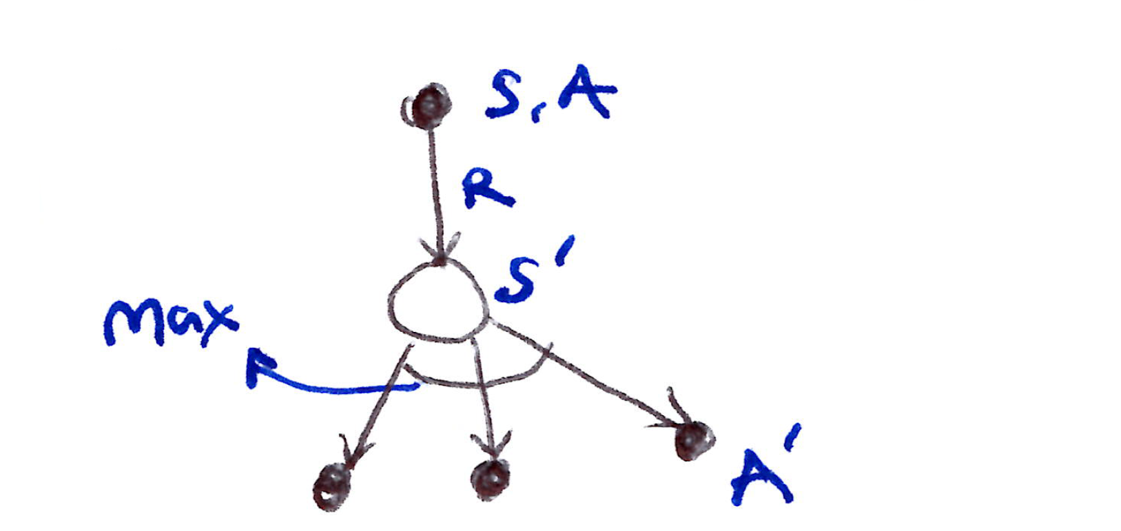
Q-learning backup diagram: from state-action (S, A) through reward R to next state S', with a max over all next actions A'.
Q-learning (Consider Off-policy Learning of Q(s,a))
- Next action is chosen using the behavior policy:
A_{t+1} \sim \mu(\cdot | S_t)
- But we consider an alternative successor action A' \sim \pi(\cdot | S_t) and update Q(S_t, A_t) towards the value of that alternative action, as seen in the update equation:
Q(S_t, A_t) \leftarrow Q(S_t, A_t) + \alpha\Big[\underbrace{R_{t+1} + \gamma Q(S_{t+1}, A')}_{\text{Q-learning target}} - Q(S_t, A_t)\Big]
- Employs value iteration.
Off-policy Control with Q-learning
- We improve both policies (target & behavior):
- Improve target policy \pi greedily w.r.t. Q(s,a): \pi(S_{t+1}) = \arg\max_{a'} Q(S_{t+1}, a')
- Improve behavior policy \mu \boldsymbol{\varepsilon}-greedily w.r.t. Q(s,a)
- The Q-learning target then simplifies:
R_{t+1} + \gamma Q(S_{t+1}, A') = R_{t+1} + \gamma Q\!\left(S_{t+1}, \arg\max_{a'} Q(S_{t+1}, a')\right) = R_{t+1} + \gamma \max_{a'} Q(S_{t+1}, a')
Pseudocode: Q-learning for estimating \pi \approx \pi_*
\boxed{ \begin{aligned} &\textbf{Algorithm parameters: } \alpha \in (0,1]\text{, small } \varepsilon > 0 \\ &\textbf{Initialize } Q(s,a) \text{ for all } s \in \mathcal{S}^+\text{, } a \in \mathcal{A}(s)\text{, arbitrarily except that } Q(\text{terminal}, \cdot) = 0 \\ &\textbf{Loop for each episode:} \\ &\quad \text{Initialize } S \\ &\quad \textbf{Loop for each step of episode:} \\ &\qquad \text{Choose } A \text{ from } S \text{ using policy derived from } Q \text{ (e.g. } \varepsilon\text{-greedy)} \\ &\qquad \text{Take action } A\text{, observe } R, S' \\ &\qquad Q(S,A) \leftarrow Q(S,A) + \alpha\!\left[R + \gamma \max_a Q(S',a) - Q(S,A)\right] \\ &\qquad S \leftarrow S' \\ &\quad \textbf{Until } S \text{ is terminal} \end{aligned} }
6.6 Expected Sarsa
- Instead of updating Q(S,A) with the value maximising action at S_{t+1}, \max_a Q(S_{t+1}, a) as used in Q-learning, or the \varepsilon-greedy exploratory action as in SARSA, we can use the expected value of Q at S_{t+1}, taking into account how likely each action is under the current policy. The update rule is:
\boxed{\begin{aligned} Q(S_t, A_t) &\leftarrow Q(S_t, A_t) + \alpha\left[R_{t+1} + \gamma\, \mathbb{E}_\pi\left[Q(S_{t+1}, A_{t+1}) \vert S_{t+1}\right] - Q(S_t, A_t)\right] \\[6pt] Q(S_t, A_t) &\leftarrow Q(S_t, A_t) + \alpha\left[R_{t+1} + \gamma \sum_a \pi(a \vert S_{t+1})\, Q(S_{t+1}, a) - Q(S_t, A_t)\right] \end{aligned}}
- Given the next state S_{t+1}, this algorithm moves deterministically in the same direction as SARSA moves in expectation, hence the name Expected SARSA.
- Expected SARSA eliminates the variance due to the random selection of A_{t+1}.
- Given the same amount of experience, Expected SARSA generally performs better than SARSA.
- Expected SARSA is an on-policy learning method, but if we change our target policy such that \pi is the greedy policy while our behavior is more exploratory, then it becomes an off-policy algorithm.
- Expected SARSA becomes Q-learning if \pi is the greedy policy and our behavior policy (\mu) is more exploratory (\varepsilon-greedy).
- Essentially, it is a generalization of Q-learning that has a reliable improvement over SARSA.
6.7 Maximization Bias & Double Learning
- All the control algorithms discussed so far utilize maximization operations in target policy constructions (\varepsilon-greedy or greedy action selection).
- This implicitly favors positive numbers (significant positive bias).
- If the true values of state-action pairs q(s,a) of a single state s with multiple actions a are all zero, i.e. q(s,a) = 0\ \forall s, a, but whose estimated values Q(s,A) are uncertain and thus distributed some above & some below zero, then the maximum of the true values is zero, but the maximum of the estimates is positive; hence a positive bias.
- This is called the maximization bias:
\begin{aligned} q(s,a) = 0 \quad \forall s,a &\implies \max_{s,a} q(s,a) = 0 \\[6pt] Q(s,a) = \left\{ \begin{array}{l} \geq 0 \\ < 0 \end{array} \right\} &\implies \max_{s,a} Q(s,a) > 0 \end{aligned}
We can avoid maximization bias by learning 2 independent estimates of the value function Q_1(a), Q_2(a), in which we could then:
- Use one estimate, e.g. Q_1, to determine the maximizing action: \quad A^* = \arg\max_a Q_1(a)
- Then use the other, Q_2, to estimate its value: \quad Q_2(A^*) = Q_2(\arg\max_a Q_1(a))
This idea is called Double Learning.
- It doubles the memory requirements, but does not increase the amount of computation per step.
The Q-value estimate is unbiased in the sense that \mathbb{E}\left[Q_2(A^*)\right] = q(A^*).
Double Learning for Q-learning is called Double Q-learning.
Pseudocode: Double Q-learning for estimating Q_1 \approx Q_2 \approx q_*
\boxed{ \begin{aligned} &\textbf{Algorithm parameters: } \alpha \in (0,1]\text{, small } \varepsilon > 0 \\ &\textbf{Initialize } Q_1(s,a)\ \&\ Q_2(s,a) \text{ for all } s \in \mathcal{S}^+\text{, } a \in \mathcal{A}(s) \text{ s.t. } Q(\text{terminal}, \cdot) = 0 \\ &\textbf{Loop for each episode:} \\ &\quad \text{Initialize } S \\ &\quad \textbf{Loop for each step of episode:} \\ &\qquad \text{Choose } A \text{ from } S \text{ using } \varepsilon\text{-greedy policy in } Q_1 + Q_2 \\ &\qquad \text{Take action } A\text{, observe } R, S' \\ &\qquad \text{With probability } 0.5\text{:} \\ &\qquad\quad Q_1(S,A) \leftarrow Q_1(S,A) + \alpha\!\left[R + \gamma Q_2\!\left(S',\, \arg\max_a Q_1(S',a)\right) - Q_1(S,A)\right] \\ &\qquad \text{else:} \\ &\qquad\quad Q_2(S,A) \leftarrow Q_2(S,A) + \alpha\!\left[R + \gamma Q_1\!\left(S',\, \arg\max_a Q_2(S',a)\right) - Q_2(S,A)\right] \\ &\qquad S \leftarrow S' \\ &\quad \textbf{Until } S \text{ is terminal} \end{aligned} }
Double Q-learning Update Rule:
\boxed{Q_1(S_t, A_t) \leftarrow Q_1(S_t, A_t) + \alpha\left[R_{t+1} + \gamma\, Q_2\!\left(S_{t+1},\, \arg\max_a Q_1(S_{t+1}, a)\right) - Q_1(S_t, A_t)\right]}
6.8 Games, Afterstates & Other Special Cases
- Our general approach so far revolves around learning an action-value function, where the value of an action in a given state is quantified/evaluated before the action is taken.
- In some specialized cases, it is expedient to evaluate the value function after an action.
- The state-value function that evaluates states after the action are referred to as afterstates & the value functions over these afterstates are called the afterstate value functions.
- This is the case in Tic-tac-toe and chess (evaluate board position after agent has made its move).
- Afterstates are useful when we have partial knowledge (initial part) of the environment’s dynamics but not full dynamics.
- It is also useful where many different actions may lead to the same state afterward.
- Afterstate methods are aptly described in terms of GPI, with a policy and afterstate value function interacting in essentially the same way.
- Still have to decide between on or off policy for managing the need for persistent exploration.
6.9 Summary
- TD methods learn from incomplete episodes and are alternatives to MC methods for solving the prediction part of the RL problem.
- They use GPI to solve the control part of the RL problem.
- When issues arise with maintaining sufficient exploration in prediction, TD control methods deal with this issue via an on-policy or off-policy approach:
- Sarsa (on-policy)
- Q-learning (off-policy)
- Expected Sarsa (off-policy)
- The TD methods used here in this chapter should be rightly called one-step, tabular, model-free TD methods.