5 Monte Carlo Methods
- Monte Carlo methods are used when we do not have knowledge of the transition probabilities (model of the environment) and then we must learn directly from experience (model-free).
- Learning from actual experience is striking because it requires no prior knowledge of the environment’s dynamics, yet can still attain optimal behavior.
- Experience: sample sequences of states, actions, and rewards from actual/simulated interaction with an environment.
- Monte Carlo methods are only applied to episodic tasks.
- MC methods estimate the value function of an unknown MDP by learning the value function from samples instead of computing from knowledge of the MDP.
- We use Generalized Policy Iteration (GPI), developed in Ch. 4, to handle the nonstationarity.
- First consider the prediction problem (computation of V_\pi & q_\pi for a fixed arbitrary policy \pi), then policy improvement, and finally the control problem and its solution by GPI.
5.1 Monte Carlo Prediction
Recall that the value of a state is the expected cumulative future discounted reward (expected return). An obvious way of estimating that value from experience is to simply average the returns observed after visits to that state. As more returns are observed, the average should converge to the expected value. This idea underlies all Monte Carlo methods.
MC uses the simplest possible idea: Value = mean return
MC learns from complete episodes: no bootstrapping
MC is model-free: no knowledge of MDP transitions/rewards
Goal: Learn v_\pi from episodes of experience under policy \pi
S_1, A_1, R_2, \ldots, S_K \sim \pi
Value function (expected return):
v_\pi(s) = \mathbb{E}\left[G_t \mid S_t = s\right]
Return (total discounted reward):
G_t = R_{t+1} + \gamma R_{t+2} + \gamma^2 R_{t+3} + \ldots + \gamma^{T-1} R_T
The 2 Monte Carlo methods are First-Visit & Every-Visit MC:
- First-Visit: estimates v_\pi(s) as the average of the returns following first visits to s
- Every-Visit: estimates v_\pi(s) by averaging the returns following all visits to s
- Both methods converge to v_\pi(s) as the number of visits (or first visits) to s goes to \infty
- Every-visit MC extends more naturally to function approximation & eligibility traces
\boxed{V(S_t) \leftarrow V(S_t) + \alpha\left[G_t - V(S_t)\right]}
First-Visit or Every-Visit Monte Carlo Policy Evaluation
- To evaluate state s
- The first timestep or every timestep t that state s is visited in an episode
- Increment counter: N(s) \leftarrow N(s) + 1
- Increment total return: S(s) \leftarrow S(s) + G_t
- Value is estimated by mean return: V(s) = S(s) / N(s)
- By law of large numbers, V(s) \to V_\pi(s) as N(s) \to \infty
5.2 Monte Carlo Estimation of Action Values
Without a model, state-values are not sufficient to determine a policy. The value of each action must be explicitly estimated in order for the values to be useful in suggesting a policy.
One of the primary goals for Monte Carlo methods is to estimate the state-action value functions, q.
Issue: Many state-action pairs may never be visited under a deterministic policy \pi.
Fix: For policy evaluation to work for action values, we must assure continual exploration of the state space.
- We can do this by specifying that the episodes start in a state-action pair, and that every pair has a nonzero probability of being selected as the start. This guarantees that all state-action pairs will be visited an infinite number of times in the limit of an infinite number of episodes.
- This is called the assumption of exploring starts.
- Exploring starts fails when learning directly from actual interaction with an environment.
- A common alternative approach is to consider only policies that are stochastic with a nonzero probability of selecting all actions in each state.
5.3 Monte Carlo Control
Monte Carlo estimation can be used in control to approximate optimal policies via generalized policy iteration (GPI).
GPI diagram:
- Policy evaluation: MC policy eval, Q = q_\pi
- Policy improvement: \varepsilon-greedy policy improvement
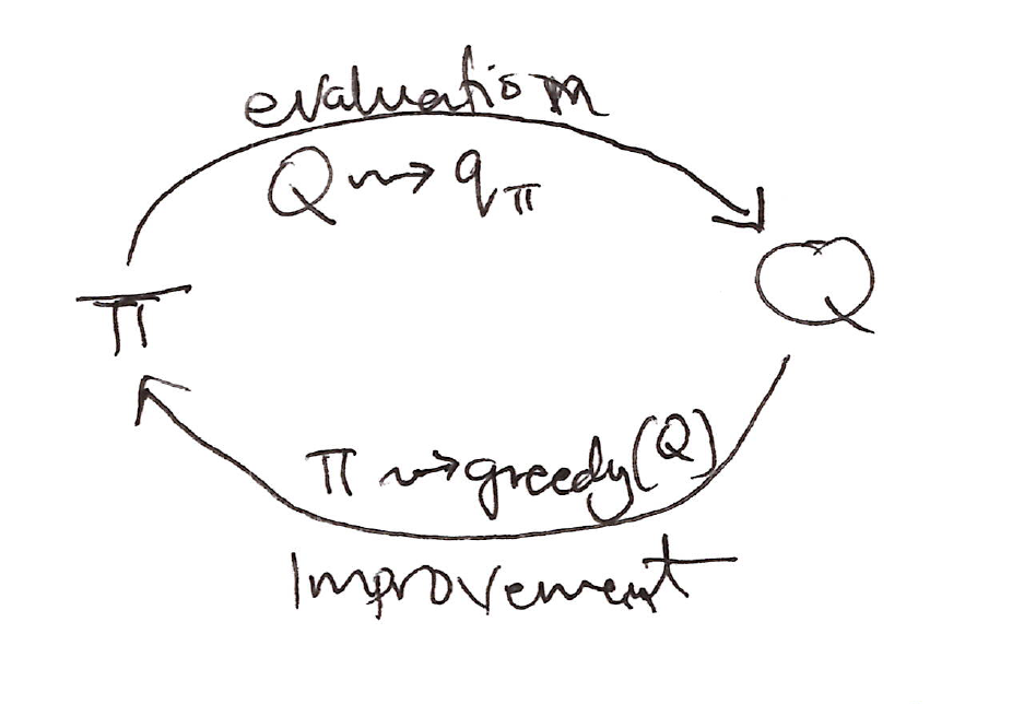
In GPI, one maintains both an approximate policy and an approximate value function.
\pi_0 \xrightarrow{E} q_{\pi_0} \xrightarrow{I} \pi_1 \xrightarrow{E} q_{\pi_1} \xrightarrow{I} \pi_2 \xrightarrow{E} \ldots \xrightarrow{I} \pi_* \xrightarrow{E} q_{\pi_*}
where \xrightarrow{E} denotes a complete policy evaluation & \xrightarrow{I} denotes a complete policy improvement.
Policy Improvement
- For q_\pi, the greedy policy \forall s \in S:
\pi(s) \doteq \arg\max_a q_\pi(s, a)
- Policy improvement theorem applied to \pi_k & \pi_{k+1} for all s \in S:
\begin{align*} q_{\pi_k}(s, \pi_{k+1}(s)) &= q_{\pi_k}\!\left(s, \arg\max_a\, q_{\pi_k}(s,a)\right) \\ &= \max_a\, q_{\pi_k}(s,a) \\ &\geq q_{\pi_k}(s, \pi_k(s)) \\ &\geq v_{\pi_k}(s) \end{align*}
- The idea of GPI is to avoid the infinite number of episodes nominally required for policy evaluation. This is value iteration.
- Only one iteration of iterative policy evaluation is performed between each step of policy improvement.
- For a deterministic policy for control, it’s essential we use exploring starts to ensure sufficient exploration. This creates the Monte Carlo ES Algorithm.
- This is inefficient because, for each state-action pair, it maintains a list of all returns & repeatedly calculates their mean.
- More efficient would be to maintain just the mean & count for each state-action pair and update them incrementally.
5.4 Monte Carlo Control Without Exploring Starts
How can we avoid the unlikely assumption of exploring starts? (unrealistic assumption)
To avoid having to use exploring starts, we can use two approaches, on-policy and off-policy methods. These are the only ways to ensure that all actions are selected infinitely often by the agent continuing to select them.
- On-policy: Evaluate/improve the policy that is used to make the decisions
- Learn about policy \pi from experience sampled from \pi
- Uses \varepsilon-greedy policy; generally soft policy (assign nonzero probability to each possible action): \pi(a|s) > 0\ \quad \forall s \in S,\ a \in A(s)
- Off-policy: Evaluate/improve a policy different from that used to generate the data
- Learn about target policy \pi from experience sampled from behavior policy \mu
- On-policy: Evaluate/improve the policy that is used to make the decisions
\varepsilon-greedy Exploration
\pi(a \vert s) = \left\{ \begin{array}{ll} 1 - \varepsilon + \dfrac{\varepsilon}{\vert A(s) \vert} & \text{if greedy action} \\[6pt] \dfrac{\varepsilon}{\vert A(s) \vert} & \text{if non-greedy action} \end{array} \right\}
\varepsilon-greedy Policy Improvement
- For any \varepsilon-soft policy \pi, any \varepsilon-greedy policy w.r.t. q_\pi is guaranteed to be better than or equal to \pi.
- For any \varepsilon-soft policy \pi, any \varepsilon-greedy policy \pi' w.r.t. q_\pi is an improvement: v_{\pi'}(s) \geq v_\pi(s)
\begin{align*} q_{\pi}(s, \pi'(s)) &= \sum_a \pi'(a \vert s)\, q_{\pi}(s,a) \\[6pt] &= \frac{\varepsilon}{\vert A(s) \vert} \sum_a q_{\pi}(s,a) + (1-\varepsilon) \max_a q_{\pi}(s,a) \\[6pt] &\geq \frac{\varepsilon}{\vert A(s) \vert} \sum_a q_{\pi}(s,a) + (1-\varepsilon) \sum_a \frac{\pi(a \vert s) - \frac{\varepsilon}{\vert A(s) \vert}}{1-\varepsilon}\, q_{\pi}(s,a) \\[6pt] &= \frac{\varepsilon}{\vert A(s) \vert} \sum_a q_{\pi}(s,a) + \sum_a \pi(a \vert s)\, q_{\pi}(s,a) - \frac{\varepsilon}{\vert A(s) \vert} \sum_a q_{\pi}(s,a) \\[6pt] &= \sum_a \pi(a \vert s)\, q_{\pi}(s,a) \\[6pt] &= v_{\pi}(s) \end{align*}
By the policy improvement theorem, \pi' \geq \pi (i.e., v_{\pi'}(s) \geq v_\pi(s) for all s \in S).
A policy \pi is optimal among \varepsilon-soft policies if and only if v_\pi = \tilde{v}_*
\tilde{v}_* is the unique solution to the Bellman optimality equation with altered transition probabilities:
\begin{align*} \tilde{v}_{*}(s) &= \max_a \sum_{s',r} \left[(1-\varepsilon)\,p(s',r \vert s,a) + \sum_{a'} \frac{\varepsilon}{\vert A(s) \vert}\, p(s',r \vert s,a')\right]\left[r + \gamma \tilde{v}_{*}(s')\right] \\[8pt] &= (1-\varepsilon) \max_a \sum_{s',r} p(s',r \vert s,a)\left[r + \gamma \tilde{v}_{*}(s')\right] + \frac{\varepsilon}{\vert A(s) \vert} \sum_a \sum_{s',r} p(s',r \vert s,a)\left[r + \gamma \tilde{v}_{*}(s')\right] \end{align*}
- When equality holds and the \varepsilon-soft policy \pi is no longer improved, then:
\begin{align*} v_{\pi}(s) &= (1-\varepsilon) \max_a q_{\pi}(s,a) + \frac{\varepsilon}{\vert A(s) \vert} \sum_a q_{\pi}(s,a) \\[8pt] &= (1-\varepsilon) \max_a \sum_{s',r} p(s',r \vert s,a)\left[r + \gamma v_{\pi}(s')\right] + \frac{\varepsilon}{\vert A(s) \vert} \sum_a \sum_{s',r} p(s',r \vert s,a)\left[r + \gamma v_{\pi}(s')\right] \end{align*}
- Because \tilde{v}_* is the unique solution, it must be that v_\pi = \tilde{v}_*.
5.5 Off-Policy Prediction via Importance Sampling
A huge dilemma is faced when learning control:
- The need to find the optimal policy, but can only do so by behaving non-optimally in order to explore all actions.
- On-policy was a compromise; it learns action values not for the optimal policy, but for a near-optimal policy that still explores.
How can learning control methods learn about the optimal policy while behaving according to an exploratory policy?
An off-policy learning uses 2 policies:
- A behavior policy (used to generate the data; action)
- A target policy (for control; becomes the optimal policy)
Off-policy learning methods are more powerful and general than on-policy methods.
Let’s consider the prediction problem, in which both target & behavior policies are fixed and given.
- Goal: Estimate v_\pi or q_\pi, but all we have are episodes following another policy b, where b \neq \pi
- \pi \equiv target policy
- b \equiv behavior policy
- Goal: Estimate v_\pi or q_\pi, but all we have are episodes following another policy b, where b \neq \pi
In order to use episodes from b to estimate values for \pi, we require that every action taken under \pi is also taken, at least occasionally, under b, i.e.,:
\pi(a|s) > 0 \implies b(a|s) > 0
This is called the assumption of coverage.
It follows from coverage that:
- b must be stochastic in states where it is not identical to \pi
- \pi may be deterministic
Almost all off-policy methods use importance sampling, a general technique for estimating expected values under one distribution given samples from another.
Given a starting state S_t, the probability of the subsequent state-action trajectory, A_t, S_{t+1}, A_{t+1}, \ldots, S_T, occurring under any policy \pi is:
\begin{align*} &\Pr\{A_t, S_{t+1}, A_{t+1}, \ldots, S_T \mid S_t,\; A_{t:T-1} \sim \pi\} \\[8pt] &= \pi(A_t \vert S_t)\, p(S_{t+1} \vert S_t,A_t)\, \pi(A_{t+1} \vert S_{t+1}) \cdots p(S_T \vert S_{T-1},A_{T-1}) \\[8pt] &= \prod_{k=t}^{T-1} \pi(A_k \vert S_k)\, p(S_{k+1} \vert S_k, A_k) \end{align*}
\begin{aligned} \text{where } p &\equiv \text{state-transition probability function} \end{aligned}
- The relative probability of the trajectory under the target and behavior policies (the importance-sampling ratio) is:
\boxed{\rho_{t:T-1} \doteq \frac{\prod_{k=t}^{T-1} \pi(A_k|S_k)\, p(S_{k+1}|S_k,A_k)}{\prod_{k=t}^{T-1} b(A_k|S_k)\, p(S_{k+1}|S_k,A_k)} = \prod_{k=t}^{T-1} \frac{\pi(A_k|S_k)}{b(A_k|S_k)}}
The state transition probability functions cancel out in the numerator & denominator.
We want to estimate the expected returns (values) under the target policy, but all we have are returns G_t due to the behavior policy.
- To address this we simply multiply expected returns from the behavior policy by the importance sampling ratio to get the value function for our target policy:
\mathbb{E}\left[\rho_{t:T-1}\, G_t \mid S_t = s\right] = v_\pi(s)
- MC algorithm that averages returns from a batch of observed episodes following policy b to estimate v_\pi(s):
- \mathcal{T}(s) \equiv set of all time steps in which state s is visited
- T(t) \equiv 1st time of termination following time t
- G_t \equiv return after t up through T(t)
- \{G_t\}_{t \in \mathcal{T}(s)} \equiv returns that pertain to state s
- \{\rho_{t:T-1}\}_{t \in \mathcal{T}(s)} \equiv corresponding importance-sampling ratios
Ordinary importance sampling (unbiased): \boxed{V(s) \doteq \frac{\sum_{t \in \mathcal{T}(s)} \rho_{t:T(t)-1}\, G_t}{|\mathcal{T}(s)|}}
Weighted importance sampling (biased): \boxed{V(s) \doteq \frac{\sum_{t \in \mathcal{T}(s)} \rho_{t:T(t)-1}\, G_t}{\sum_{t \in \mathcal{T}(s)} \rho_{t:T(t)-1}}}
5.6 Incremental Implementation
Monte Carlo prediction methods can be implemented incrementally, on an episode-by-episode basis like the way we did in Chapter 2 (Section 2.4).
General form:
\text{NewEstimate} \leftarrow \text{OldEstimate} + \text{StepSize}\left[\text{Target} - \text{OldEstimate}\right]
- Suppose we have a sequence of returns G_1, G_2, \ldots, G_{n-1}, all starting in the same state and each with a corresponding random weight W_i (e.g. W_i = \rho_{t_i:T(t_i)-1}). We wish to form the estimate, V_n, and keep it up-to-date as we obtain a single additional return G_n:
V_n \doteq \frac{\sum_{k=1}^{n-1} W_k G_k}{\sum_{k=1}^{n-1} W_k}, \quad n \geq 2
In addition to keeping track of V_n, we must maintain for each state the cumulative sum C_n of the weights given to the first n returns.
The update rule for V_n is:
\begin{aligned} V_{n+1} &\doteq V_n + \frac{W_n}{C_n}\left[G_n - V_n\right], \quad n \geq 1 \\[6pt] C_{n+1} &\doteq C_n + W_{n+1} \end{aligned}
\begin{aligned} \text{where } C_0 \doteq 0 \text{ and } V_1 \to \text{arbitrary.} \end{aligned}
5.7 Off-Policy Monte Carlo Control
- Using incremental implementation and importance sampling, we can now discuss off-policy Monte Carlo control (follows the behavior policy while learning about and improving the target policy).
- To explore all possibilities, we require that the behavior policy be soft (i.e., that it selects all actions in all states with nonzero probability).
- Off-policy Monte Carlo control method based on GPI and weighted importance sampling for estimating \pi_* & q_*:
- The target policy \pi \approx \pi_* is the greedy policy w.r.t. Q, which is an estimate of q_\pi
- The behavior policy b can be anything, but in order to assure convergence of \pi to \pi_*, an infinite number of returns must be obtained for each state-action pair.
- This can be assured by choosing b to be an \varepsilon-soft policy.
5.8 Discounting-aware Importance Sampling
So far our off-policy methods consider returns as unitary wholes, without taking into account the returns’ internal structures as sums of discounted rewards.
Let’s think of discounting as determining a probability of termination, or equivalently a degree of partial termination \gamma \in (0,1]; T \equiv\text{time of termination of the episode}
The flat partial returns:
\boxed{\bar{G}_{t:h} \doteq R_{t+1} + R_{t+2} + \ldots + R_h, \quad 0 \leq t \leq h \leq T}
\begin{aligned} \text{where "flat"} &\equiv \text{absence of discounting} \\[6pt] \text{"partial"} &\equiv \text{these returns do not extend all the way to termination,} \\ &\quad \text{but instead stop at } h, \text{ called the \textbf{horizon}} \end{aligned}
- The conventional full return G_t can be viewed as a sum of flat partial returns:
\begin{aligned} G_t &= R_{t+1} + \gamma R_{t+2} + \gamma^2 R_{t+3} + \ldots + \gamma^{T-t-1} R_T \\[6pt] &= (1-\gamma) R_{t+1} + \gamma(1-\gamma)(R_{t+1} + R_{t+2}) + (1-\gamma)\gamma^2(R_{t+1} + R_{t+2} + R_{t+3}) \\ &\quad + \ldots + (1-\gamma)\gamma^{T-t-2}(R_{t+1} + R_{t+2} + \ldots + R_{T-1}) + \gamma^{T-t-1}(R_{t+1} + \ldots + R_T) \\[6pt] &= (1-\gamma)\sum_{h=t+1}^{T-1} \gamma^{h-t-1}\, \bar{G}_{t:h} + \gamma^{T-t-1}\, \bar{G}_{t:T} \end{aligned}
- Now we need to scale the flat partial returns by an importance sampling ratio that is similarly truncated:
Ordinary importance-sampling estimator:
\boxed{V(s) \doteq \frac{\sum_{t \in \mathcal{T}(s)} \left[(1-\gamma)\sum_{h=t+1}^{T(t)-1} \gamma^{h-t-1}\, \rho_{t:h-1}\, \bar{G}_{t:h} + \gamma^{T(t)-t-1}\, \rho_{t:T(t)-1}\, \bar{G}_{t:T(t)}\right]}{|\mathcal{T}(s)|}}
Weighted importance-sampling estimator:
\boxed{V(s) \doteq \frac{\sum_{t \in \mathcal{T}(s)} \left[(1-\gamma)\sum_{h=t+1}^{T(t)-1} \gamma^{h-t-1}\, \rho_{t:h-1}\, \bar{G}_{t:h} + \gamma^{T(t)-t-1}\, \rho_{t:T(t)-1}\, \bar{G}_{t:T(t)}\right]}{\sum_{t \in \mathcal{T}(s)} \left[(1-\gamma)\sum_{h=t+1}^{T(t)-1} \gamma^{h-t-1}\, \rho_{t:h-1} + \gamma^{T(t)-t-1}\, \rho_{t:T(t)-1}\right]}}
- Both estimators are called “discounting-aware” importance sampling estimators.
5.9 Per-decision Importance Sampling
- Another way to account for the structure of the return as a sum of rewards in off-policy importance sampling that may be able to reduce variance even in the absence of discounting (i.e., even if \gamma = 1):
\begin{aligned} \rho_{t:T-1}\, G_t &= \rho_{t:T-1}\left(R_{t+1} + \gamma R_{t+2} + \ldots + \gamma^{T-t-2} R_T\right) \\[6pt] &= \rho_{t:T-1}\, R_{t+1} + \gamma\, \rho_{t:T-1}\, R_{t+2} + \ldots + \gamma^{T-t-1}\, \rho_{t:T-1}\, R_T \\[10pt] \rho_{t:T-1}\, R_{t+1} &= \frac{\pi(A_t \vert S_t)}{b(A_t \vert S_t)} \cdot \frac{\pi(A_{t+1} \vert S_{t+1})}{b(A_{t+1} \vert S_{t+1})} \cdots \frac{\pi(A_{T-1} \vert S_{T-1})}{b(A_{T-1} \vert S_{T-1})}\, R_{t+1} \\[10pt] \mathbb{E}\left[\frac{\pi(A_k \vert S_k)}{b(A_k \vert S_k)}\right] &\doteq \sum_a b(a \vert S_k)\, \frac{\pi(a \vert S_k)}{b(a \vert S_k)} = \sum_a \pi(a \vert S_k) = 1 \\[10pt] \mathbb{E}\left[\rho_{t:T-1}\, R_{t+1}\right] &= \mathbb{E}\left[\rho_{t:t}\, R_{t+1}\right] \\[6pt] \mathbb{E}\left[\rho_{t:T-1}\, R_{t+k}\right] &= \mathbb{E}\left[\rho_{t:t+k-1}\, R_{t+k}\right] \\[6pt] \mathbb{E}\left[\rho_{t:T-1}\, G_t\right] &= \mathbb{E}\left[\tilde{G}_t\right] \end{aligned}
\text{where: } \quad \tilde{G}_t = \rho_{t:t}\, R_{t+1} + \gamma\, \rho_{t:t+1}\, R_{t+2} + \gamma^2\, \rho_{t:t+2}\, R_{t+3} + \ldots + \gamma^{T-t-1}\, \rho_{t:T-1}\, R_T
Ordinary importance-sampling estimator using \tilde{G}_t (lower variance expectation):
\boxed{V(s) \doteq \frac{\sum_{t \in \mathcal{T}(s)} \tilde{G}_t}{|\mathcal{T}(s)|}}
5.10 Summary
- Monte Carlo (MC) methods covered so far learn value functions and optimal policies from experience in the form of sample episodes, which lead to at least 3 kinds of advantages over DP methods for MC methods:
- Learn optimal behavior directly from interaction with the environment (model-free)
- Can be used with simulation or sample models
- Are easier and more efficient to focus on a small subset of the states
- Are less harmed by violations of the Markov property (no bootstrapping)
- In Chapter 4, we followed GPI overall schema in designing MC control methods.
- MC methods provide an alternative policy evaluation process, using average of many returns that start in each state as a good approximator for that state value’s expected return.
- MC methods intermix policy evaluation and policy improvement steps on an episode-by-episode basis, and can be incrementally implemented on an episode-by-episode basis.
- Maintaining sufficient exploration is an issue in MC control methods.
- One fix is by assuming that episodes begin with state-action pairs randomly selected to cover all possibilities. These are called exploring starts.
- On-policy methods utilize one policy for both action and target selection.
- Off-policy methods use a different behavior policy from the deterministic target policy.
- Off-policy prediction refers to learning the value function of a target policy from data generated by a different behavior policy.
- These learning methods are based on some form of importance sampling, i.e., on weighting returns by the ratio of the probabilities of taking the observed actions under the 2 different policies, thereby transforming their expectations from the behavior policy to the target policy.
- Ordinary importance sampling uses a simple average of the weighted returns (unbiased estimates)
- Weighted importance sampling uses a weighted average (biased estimates)
- These learning methods are based on some form of importance sampling, i.e., on weighting returns by the ratio of the probabilities of taking the observed actions under the 2 different policies, thereby transforming their expectations from the behavior policy to the target policy.
- The MC methods in this chapter differ from the DP methods in Chapter 4 in 2 key ways:
- They operate on sample experience, and thus can be used for direct learning without a model.
- They do not bootstrap (no update of value estimates on the basis of other value estimates).
- In chapter 6, we’ll consider methods that learn from experience, like MC methods, but also bootstrap, like DP methods.