4  Dynamic Programming

Dynamic Programming (DP): A collection of algorithms that can be used to compute optimal policies given a perfect model of the environment as an MDP.

Assumptions:

1. The environment is a finite MDP
2. State S, action A, and reward R sets are finite
   • Its dynamics are given by a set of probabilities p(s', r | s, a) for all s \in S, a \in A(s), r \in R, s' \in S^+ (S^+ is S plus a terminal state if the problem is episodic)

p(s', r | s, a) = \mathbb{P}\left[R_{t+1} = r,\, S_{t+1} = s' \mid S_t, A_t\right]

Key idea:

• Use value functions to organize & structure the search for good policies
• Show how DP can be used to compute the value functions
• v_* or q_* that satisfy the Bellman Optimality Equations can then be used to easily obtain optimal policies \pi_*

Bellman Optimality Equations

\quad \forall s \in S,\, a \in A(s),\, s' \in S^+

• State-Value function:

\begin{align*} v_{*}(s) &= \max_a\, \mathbb{E}\left[R_{t+1} + \gamma v_{*}(S_{t+1}) \mid S_t = s,\, A_t = a\right] \\ &= \max_a \sum_{s', r} p(s', r \vert s, a)\left[r + \gamma v_{*}(s')\right] \end{align*}

• Action-Value function:

\begin{align*} q_{*}(s,a) &= \mathbb{E}\left[R_{t+1} + \gamma \max_{a'} q_{*}(S_{t+1}, a') \mid S_t = s,\, A_t = a\right] \\ &= \sum_{s', r} p(s', r \vert s, a)\left[r + \gamma \max_{a'} q_{*}(s', a')\right] \end{align*}

---

4.1 Policy Evaluation (Prediction)

Policy Evaluation: How to compute the state-value function v_\pi for an arbitrary policy \pi.

\begin{align*} v_\pi(s) &\doteq \mathbb{E}\left[G_t \mid S_t = s\right] \\ &= \mathbb{E}_\pi\left[R_{t+1} + \gamma G_{t+1} \mid S_t = s\right] \\ &= \mathbb{E}_\pi\left[R_{t+1} + \gamma v_\pi(S_{t+1}) \mid S_t = s\right] \\ &= \sum_a \pi(a \vert s) \sum_{s', r} p(s', r \vert s, a)\left[r + \gamma v_\pi(s')\right] \end{align*}

• If the dynamics are known perfectly/completely, then the equation above becomes a system of |S| simultaneous linear equations in |S| unknowns, where the unknowns are v_\pi(s),\ s \in S.

• If we consider an iterative sequence of approximate value functions (v_0, v_1, v_2, \ldots): S^+ \Rightarrow \mathbb{R} with initial approximation v_0 chosen arbitrarily, then each successive approximation is obtained by using the Bellman Equation for v_\pi as an update rule, \forall s \in S:

\begin{align*} v_{k+1}(s) &\doteq \mathbb{E}_\pi\left[R_{t+1} + \gamma v_k(S_{t+1}) \mid S_t = s\right] \\ &= \sum_a \pi(a \vert s) \sum_{s', r} p(s', r \vert s, a)\left[r + \gamma v_k(s')\right] \end{align*}

Iterative Policy Evaluation

• Eventually \{v_k\} sequence converges to v_\pi as k \to \infty under the same conditions that guarantee the existence of v_\pi. This is iterative policy evaluation.
• At each iteration k+1, for all states s \in S, we update v_{k+1}(s) from v_k(s') where s' is a successor state of s.
• This update is called an expected update because it is based on the expectation over all possible next states, rather than a sample of reward/value from the next state.
• We think of the updates occurring through sweeps of state space.

---

4.2 Policy Improvement

\begin{align*} q_\pi(s,a) &\doteq \mathbb{E}\left[R_{t+1} + \gamma v_\pi(S_{t+1}) \mid S_t = s,\, A_t = a\right] \\ &= \sum_{s', r} p(s', r \vert s, a)\left[r + \gamma v_\pi(s')\right] \end{align*}

The process of making a new policy that improves on an original policy, by making it greedy w.r.t. the value function of the original policy.

• Given a deterministic policy, a = \pi(s)
• We can improve the policy by acting greedily: \pi'(s) = \arg\max_{a \in A} q_\pi(s,a)
• This improves the value from any state over one step (monotonic policy improvement):

q_\pi(s, \pi'(s)) = \max_{a \in A} q_\pi(s,a) \geq q_\pi(s, \pi(s)) = v_\pi(s)

• It therefore improves the value function, v_{\pi'}(s) \geq v_\pi(s):

\begin{align*} v_\pi(s) &\leq q_\pi(s, \pi'(s)) \\ &= \mathbb{E}\left[R_{t+1} + \gamma v_\pi(S_{t+1}) \mid S_t = s,\, A_t = \pi'(s)\right] \\ &= \mathbb{E}_{\pi'}\left[R_{t+1} + \gamma v_\pi(S_{t+1}) \mid S_t = s\right] \\ &\leq \mathbb{E}_{\pi'}\left[R_{t+1} + \gamma q_\pi(S_{t+1}, \pi'(S_{t+1})) \mid S_t = s\right] \\ &= \mathbb{E}_{\pi'}\left[R_{t+1} + \gamma\, \mathbb{E}\left[R_{t+2} + \gamma V_\pi(S_{t+2}) \mid S_{t+1}, A_{t+1} = \pi'(S_{t+1})\right] \mid S_t = s\right] \\ &= \mathbb{E}_{\pi'}\left[R_{t+1} + \gamma R_{t+2} + \gamma^2 V_\pi(S_{t+2}) \mid S_t = s\right] \\ &\leq \mathbb{E}_{\pi'}\left[R_{t+1} + \gamma R_{t+2} + \gamma^2 R_{t+3} + \gamma^3 V_\pi(S_{t+3}) \mid S_t = s\right] \\ &\quad \vdots \\ &\leq \mathbb{E}_{\pi'}\left[R_{t+1} + \gamma R_{t+2} + \gamma^2 R_{t+3} + \gamma^3 R_{t+4} + \ldots \mid S_t = s\right] \\ &= \mathbb{E}_{\pi'}\left[\sum_{k=0}^{\infty} \gamma^k R_{t+k+1} \mid S_t = s\right] \\ &= \mathbb{E}_{\pi'}\left[G_t \mid S_t = s\right] \\ &= v_{\pi'}(s) \end{align*}

\therefore\quad v_\pi(s) \leq v_{\pi'}(s)

• If improvements stop: q_\pi(s, \pi'(s)) = \max_{a \in A} q_\pi(s,a) = q_\pi(s, \pi(s)) = v_\pi(s)
• Then the Bellman optimality equation has been satisfied: v_\pi(s) = \max_{a \in A} q_\pi(s,a)
• Therefore v_\pi(s) = v_*(s)\ \forall s \in S, so \pi is an optimal policy.
• Essentially, if v_\pi(s) = v_{\pi'}(s) then v_{\pi'}(s) must be v_{*}(s) & both \pi(s) and \pi'(s) are optimal policies.
• Policy improvement thus must give a strictly better policy except when the original policy is already optimal.

---

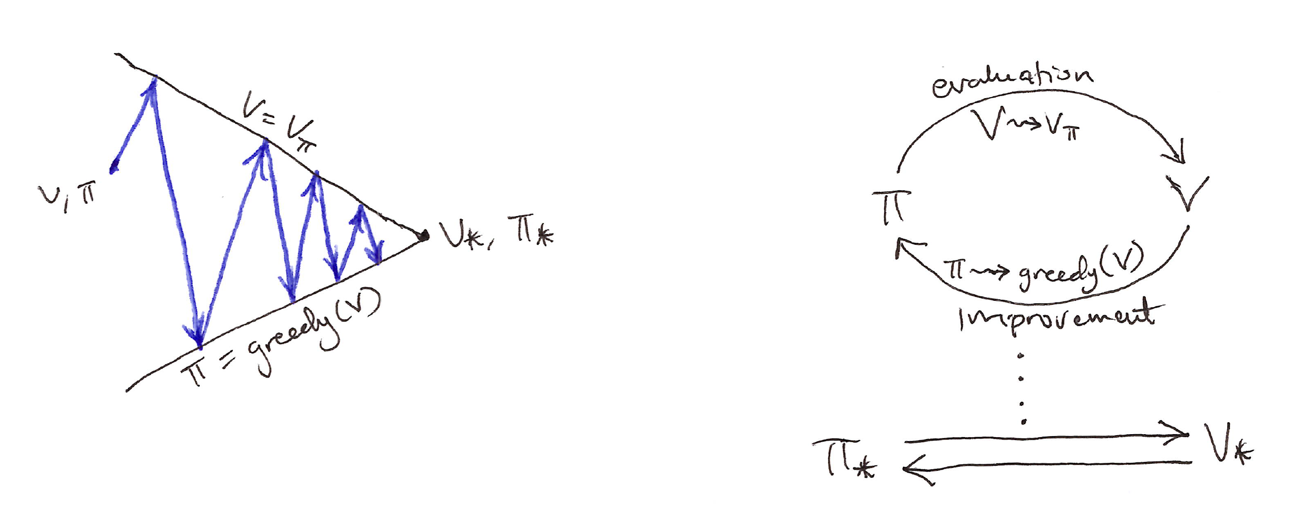
4.3 Policy Iteration

• This involves a sequence of monotonically improving policies & value functions.
• The algorithm is:
  1. Given a policy, evaluate the policy \pi to obtain the value function v_\pi
  2. Then improve the policy by acting greedily w.r.t. v_\pi to obtain new policy \pi'
  3. Evaluate new policy \pi' to obtain new value function v_{\pi'}
  4. Repeat until \pi' converges to the optimal policy \pi^{*} (only for finite MDPs)

\pi_0 \xrightarrow{E} V_{\pi_0} \xrightarrow{I} \pi_1 \xrightarrow{E} v_{\pi_1} \xrightarrow{I} \pi_2 \xrightarrow{E} \ldots \xrightarrow{I} \pi_* \xrightarrow{E} V_*

where \xrightarrow{E} denotes a policy evaluation (v_\pi(s) = \mathbb{E}_\pi\left[G_t \mid S_t = s\right]) and \xrightarrow{I} denotes a policy improvement (\pi' = \text{greedy}(v_\pi)).

• Policy iteration often converges in surprisingly few iterations.

---

4.4 Value Iteration

• Policy iteration requires full policy evaluation at each iteration step, which is a computationally expensive process that (formally) requires infinite sweeps of the state space to approach the true value function.
• Could we truncate policy evaluation without losing the convergence guarantees of policy iteration? YES
• In Value Iteration, policy evaluation is stopped after just one sweep of the state space (one update of each state).
• It can be written as a particularly simple update operation that combines the policy improvement & truncated policy evaluation steps (\forall s \in S):

\begin{align*} v_{k+1}(s) &\doteq \max_a\, \mathbb{E}\left[R_{t+1} + \gamma v_k(S_{t+1}) \mid S_t = s,\, A_t = a\right] \\ &= \max_a \sum_{s', r} p(s', r \vert s, a)\left[r + \gamma v_k(s')\right] \end{align*}

• Value iteration is obtained simply by turning the Bellman Optimality Equation into an update rule.

---

4.5 Asynchronous Dynamic Programming

• Async DP algorithms are in-place iterative DP algorithms that are not organized in terms of systematic sweeps of the state set. (localized approach)
• Async DP updates the values of states individually in any order whatsoever, using whatever values of other states happen to be available. (arbitrary order)
• 3 simple ideas for async DP:
  • In-place DP
  • Prioritized sweeping
  • Real-time DP

---

4.6 Generalized Policy Iteration (GPI)

• GPI entails letting policy evaluation and policy improvement interact, independent of the granularity & other details of the two processes.
• Both processes in GPI can be viewed as both competing & cooperating. They compete in the sense that they pull in opposing directions.

Figure 4.1: Generalized Policy Iteration

---

4.7 Efficiency of Dynamic Programming

• DP may not be practical for very large problems, but are actually quite efficient compared with other methods.
• DP is exponentially faster than any direct search in policy could be, because direct search has to be exhaustive.
• For the largest problems, only DP methods are feasible.
• DP is comparatively better suited to handling large state spaces than competing methods such as direct search and linear programming.
• Async DP methods are preferred often on problems with large state spaces.

---

4.8 Summary

• Policy Evaluation \Rightarrow (typically) iterative computation of the value functions for a given policy.

• Policy Improvement \Rightarrow computation of an improved policy given the value function for that policy.

• The combination of both computations together yields policy iteration and value iteration, the 2 most popular dynamic programming (DP) methods.

  • Either of these can be used to reliably compute optimal value functions & optimal policies for finite MDPs given complete knowledge of the MDP.

• Classical DP methods operate in sweeps through the state set, performing an expected update operation on each state.

  • Each such operation updates a single state-value on the basis of all possible successor states and their probabilities of occurring.
  • With no changes in value with subsequent updates, then convergence has occurred to values that satisfy the corresponding Bellman Equations.
  • There are 4 primary value functions (v_\pi, v_*, q_\pi, q_*), 4 corresponding Bellman equations, and 4 corresponding expected updates.
  • Backup diagrams give an intuitive view of the operation of DP updates.

• Generalized Policy Iteration (GPI): insight into DP methods, and almost all RL methods can be gained by viewing them as GPI.

  • GPI is the general idea of 2 interacting processes revolving around an approximate policy and an approximate value function.

• Asynchronous DP methods are in-place iterative methods that update states in an arbitrary order, perhaps stochastically determined and using out-of-date information.

  • No need for complete sweeps through the state set.

• All DP method updates estimates of the values of states based on estimates of the values of successor states.

  • This is called bootstrapping, when DP methods update estimates on the basis of other estimates.

• Next chapter entails RL methods that do not require a model and do not bootstrap; both separable properties but yet can be mixed in interesting combinations.