
How Attention Became Efficient & Scalable: KV Caching, MQA, GQA, MLA, and Sparse Attention.
- Attention mechanisms have evolved considerably to make transformer inference faster and more memory-efficient.
- These notes trace that evolution: from vanilla self-attention, through KV caching, to memory-saving variants like MQA, GQA, and MLA, and finally to sparse attention methods like SWA and Deepseek Sparse Attention (DSA).
Table of Contents
- Self-Attention
- Masked (Causal) Self-Attention
- Multi-Head Attention
- Key-Value Caching (KV Caching)
- Multi-Query Attention (MQA)
- Grouped Query Attention (GQA)
- Multihead Latent Attention (MLA)
- Sliding Window Attention (SWA)
- Deepseek Sparse Attention (DSA)
Appendix
Self-Attention
- See detailed notes on transformer and attention here.
Masked (Causal) Self-Attention
\[\text{Masked Attention}(Q,K,V) = \text{Softmax}\left(\frac{QK^T}{\sqrt{d_k}} + M\right)V\] \[\begin{aligned} \text{where} \\ M &\equiv \text{lookahead mask} \end{aligned}\]Multi-Head Attention
\[\text{head}_i = \text{Attention}(Q,K,V)\] \[\text{MHA} = \text{multi-head attention}(Q,K,V) = \text{Concat}(\text{head}_1, \text{head}_2, \dots, \text{head}_H)W_O = Z\] \[\text{OR}\] \[\begin{aligned} O_i &= \text{Attention}(Q_i, K_i, V_i) \\ O &= \text{MultiheadAttention}(Q,K,V) \\ O &= \text{Concat}(O_1, O_2, \dots) \\ \Delta X &= OW_O \end{aligned}\]Key-Value Caching (KV Caching)
- Due to masking, the transformer model can compute attention for all the tokens at the same time. This is called the prefilling stage.
- During inference, the key and value vectors from the previous tokens DO NOT change at all across multiple attention heads & all attention layers. It is therefore wasteful to recompute these vectors every time for each new token.
- A simple solution is to store the key & value vectors from previous tokens in memory, and reuse them when needed. This is known as KV caching.
- KV caching helps avoid unnecessary computation & therefore speeds up the decoding process.
- In KV caching, we DO NOT need to cache any of the previous query vectors because of the masked out entries, which have no effect on the attention output.
- KV caching is very effective but memory intensive.
Deepseek R1/V3 memory example
\[\text{Required memory} = (2)(\text{KV dim})(\text{Precision})(\#\text{Heads})(\#\text{Layers})(\text{Sequence length})\] \[= (2)(128)(2\ \text{bytes/element})(128\ \text{heads})(61\ \text{layers})(32{,}768\ \text{tokens})\] \[= 131\ \text{GB} \quad (\text{A lot of memory!!!})\]Multi-Query Attention (MQA)
- How do we reduce the memory requirements?
- In the MHA mechanism, we cannot adjust the KV dim, precision, or the number of layers, but maybe we can look at the number of heads.
- One simple idea is to reduce the number of heads for key and value matrices from $h$ to $1$. Therefore, there is only a single copy of key & value vectors for each token in a layer. This single copy of KV vectors is then shared across all attention heads. This is known as multi-query attention.
| KV cache per token | |
|---|---|
| MHA | 4 MB |
| MQA | 31 KB |
128x reduction in memory usage
- An issue with MQA, however, is that it sacrifices the ability to capture complex relationships between tokens. As a result, MQA’s performance degrades considerably compared to the original MHA.
- The drastic reduction of number of heads from $128$ to $1$ is likely the reason for the performance degradation of MQA. We can instead reduce the number of heads to a smaller value denoted as $n_g$.
Grouped Query Attention (GQA)
- Instead of the total reduction of number of heads to 1 for the key and value matrices as in MQA, GQA reduces the number of heads for the key and value matrices to a smaller value, $n_g$.
- GQA maintains the same overall pattern of attention as MHA, but collapses the number of key-value heads by sharing them across multiple query heads.
Multi-head attention (MHA) vs Grouped query attention (GQA)
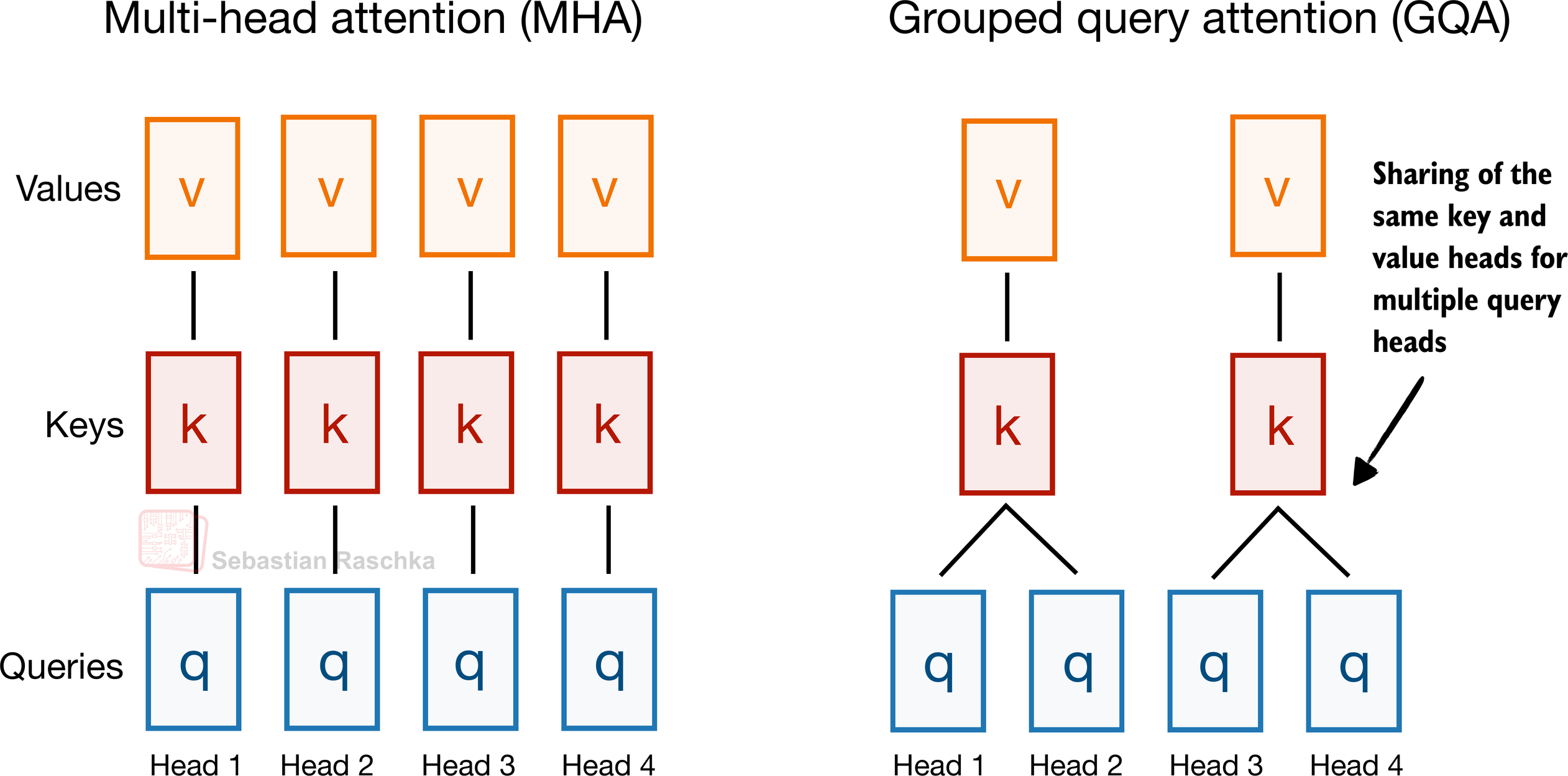
MHA: each of head₁, head₂, head₃, head₄ has its own Q, K, V.
GQA: head₁ and head₂ share one K/V pair; head₃ and head₄ share another K/V pair.
MQA: head₁, head₂, head₃, head₄ all share a single K/V pair.
- GQA strikes a balance between the memory efficiency of MQA and the expressive power of MHA.
- GQA is a popular choice in modern LLMs, including Llama 3 8B (Meta), Qwen 3 4B (Alibaba), Gemma 3 27B (Google), Mistral Small 3.1 24B (Mistral), SmolLM3 3B (Hugging Face), etc.
| KV cache per token | |
|---|---|
| MHA | 4 MB |
| MQA | 31 KB |
| GQA ($n_g = 16$) | 500 KB |
8x reduction in memory usage from MHA to GQA ($n_g = 16$)
Multihead Latent Attention (MLA)
-
See detailed notes on MLA here.
-
MLA reduces memory usage & slightly improves model performance compared to others using MHA.
-
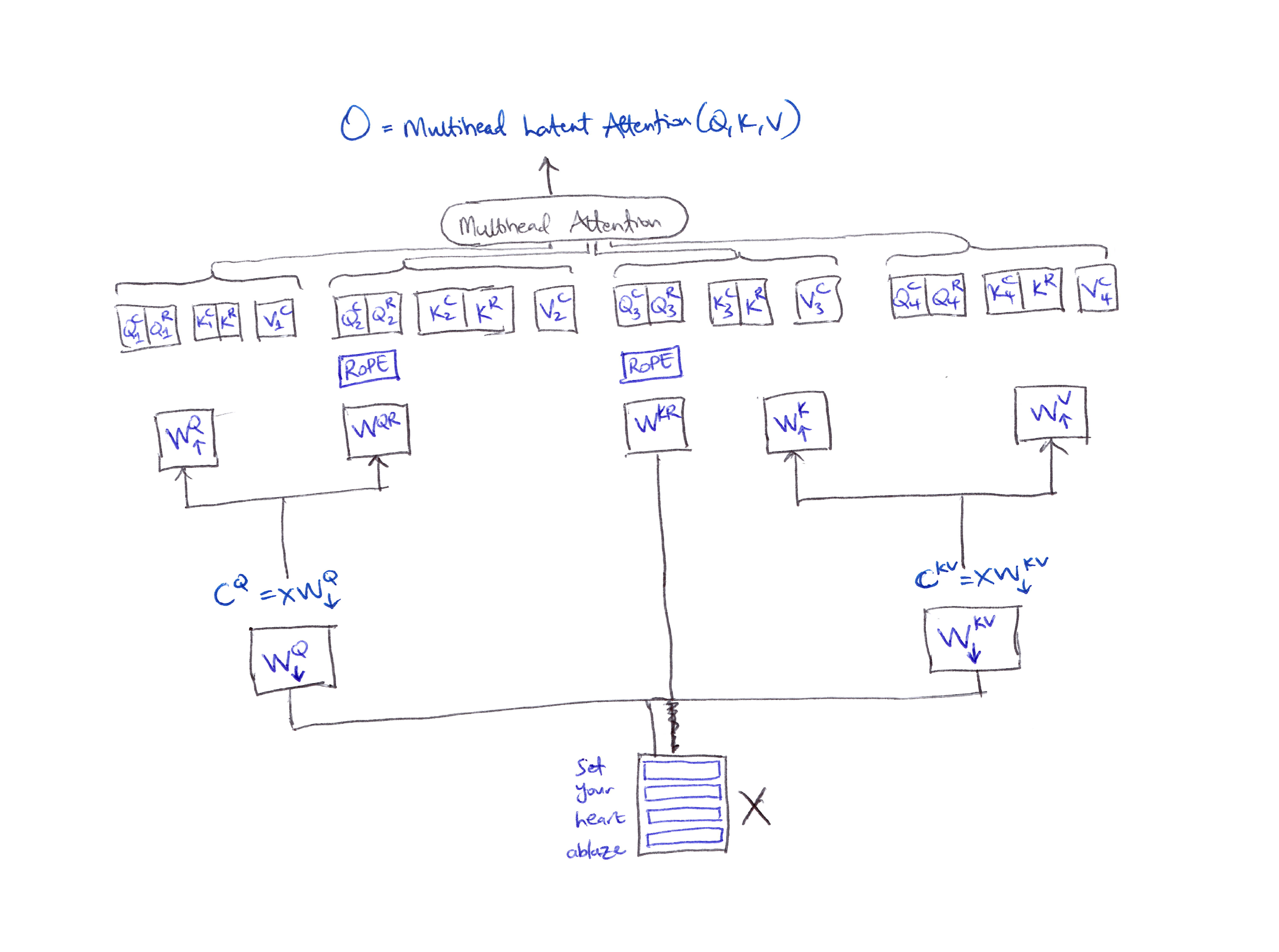
MLA compresses $Q, K, V$ representations into a low-rank space to reduce the size of the KV cache using a down-projection matrix which produces latent representations:
\[C^Q = XW^Q_\downarrow \qquad C^{KV} = XW^{KV}_\downarrow\] - These compressed latent vectors are then mapped back to $W^Q_\uparrow$, $W^K_\uparrow$, $W^V_\uparrow$ for each attention head using the corresponding up-projection matrices.
- Issue: This low-rank KV compression fails with rotary position embedding (RoPE).
- Fix: A decoupled RoPE technique which introduces extra multi-head queries $W^{QR}$ and a shared key $W^{KR}$ to encode positional information.
- For MLA, the Query, Key & Values are regrouped for each head:
- The Query is constructed by concatenating the compressed query $Q^C$ with the rotated query $Q^R$.
- The Key is constructed similarly by concatenating the compressed key $K^C$ with the rotated key $K^R$.
MLA compresses $Q, K, V$ representations into a low-rank latent space via down-projection matrices $W^Q_\downarrow$ and $W^{KV}_\downarrow$, then maps back up via up-projection matrices. A decoupled RoPE technique adds rotary queries $W^{QR}$ and a shared rotary key $W^{KR}$.
| KV cache per token | |
|---|---|
| MHA | 4 MB |
| MQA | 31 KB |
| GQA ($n_g = 16$) | 500 KB |
| MLA | 70 KB |
57x reduction in memory usage from MHA to MLA
MLA at Inference Time
\[\Delta X = OW_O = [O_1, O_2, \dots, O_h]W_O\] \[= \left[\dots, \text{Softmax}\left(\frac{Q_iK_i^T}{\sqrt{d_k}} + M\right)V_i, \dots\right]W_O\] \[\begin{aligned} Q_i &= XW_{\downarrow}^Q W_{\uparrow,i}^Q \\ K_i &= C^{KV}W_{\uparrow,i}^K = XW_{\downarrow}^{KV}W_{\uparrow,i}^K \\ V_i &= C^{KV}W_{\uparrow,i}^V \end{aligned}\] \[\begin{aligned} \text{where} \\ C^{KV} &\equiv \text{cached latent} \end{aligned}\] \[\Delta X = \left[\dots, \underbrace{\text{Softmax}\left(\frac{XW_{\downarrow}^QW_{\uparrow,i}^QW_{\uparrow,i}^{K^T}C^{KV^T}}{\sqrt{d_k}} + M\right)}_{A_i}V_i, \dots\right]W_O\] \[\Delta X = [A_1V_1, A_2V_2, \dots, A_hV_h]W_O\] \[\Delta X = \left[A_1C^{KV}W_{\uparrow,1}^V, \dots, A_hC^{KV}W_{\uparrow,h}^V\right]W_O\] \[= [A_1C^{KV}, A_2C^{KV}, A_3C^{KV}, \dots, A_hC^{KV}] \begin{bmatrix} W_{\uparrow,1}^V & 0 & 0 & \cdots & 0 \\ 0 & W_{\uparrow,2}^V & 0 & \cdots & 0 \\ 0 & 0 & W_{\uparrow,3}^V & \cdots & 0 \\ \vdots & \vdots & \vdots & \ddots & \vdots \\ 0 & 0 & 0 & \cdots & W_{\uparrow,h}^V \end{bmatrix}W_O\]Note: the up-projection matrix for the value can be incorporated into the output matrix.
- Due to the associative property, we can merge $W_{\downarrow}^QW_{\uparrow,i}^QW_{\uparrow,i}^{K^T}$ into a single matrix, which means we do not need to explicitly compute the key vectors during inference.
- Also, $W_{\uparrow}^V$ can be absorbed into $W^O$. By incorporating the up-projection matrix into the query and output matrices, we can compute attention efficiently without incurring extra computation.
- MLA has a fundamental limitation: it is incompatible with Rotary Positional Embedding (RoPE):
- We can no longer absorb the up-projection matrix $W_{\uparrow}^K$ during inference. Therefore, during inference, we must recompute the keys for all preceding tokens, which decreases inference efficiency.
- To fix this, we introduce additional multihead queries & a shared key in order to effectively encode position information when using RoPE.
- We concatenate the original query/key vectors and the rotated ones as input to the MHA computation. This approach is known as decoupled RoPE.
- MLA is used in recent LLMs such as Deepseek V3 and R1, Kimi K2, GLM-5, Ling 2.5, Mistral Large 3, Sarvam 105B, etc.
- However, as we generate more tokens, we must calculate attention between the current token and all preceding tokens. This results in slower token-per-second throughput. To fix this, Deepseek proposed a lightning indexer.
Sliding Window Attention (SWA)
- Instead of attending to the entire prefix, each token only attends to a fixed window of recent tokens around its position.
- SWA reduces the memory & compute cost of long-context inference (slower tok/s throughput) by limiting how many previous tokens each position can attend to.
- Because attention is restricted to a local token neighborhood, this mechanism is often referred to as local attention.
Regular (causal) self-attention mask vs Sliding window attention
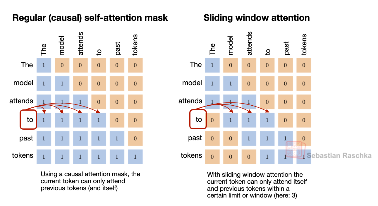
Regular (causal) self-attention mask: each token attends to all preceding tokens.
Sliding Window Attention mask (window = 3): each token attends only to itself and the previous two tokens.
Deepseek Sparse Attention (DSA)
- Deepseek proposed a lightning indexer to address the slower token-per-second throughput of MLA.
- The key concept of the lightning indexer is to quickly assess the relevance of each token and select only the most relevant ones for attention computation.
- The selected tokens are not determined by a fixed-width local window like in SWA, but by an indexer-plus-selector setup (top-k selector), where a lightning indexer computes index relevance scores, and a token selector keeps only a smaller set of high-scoring past positions 1.
- Apply partial RoPE to $W^Q$ and $W^K$ before rotation & quantization, then lightning indexing.
Quantization & Rotation in DSA
- How is the attention computation of the indexer between the query vector and all the key vectors made efficient?
- The key step is to first quantize the query & key vectors into 8-bit (BF16/FP32 → FP8) representation.
- Quantization offers a coarse approximation, greatly speeding up the calculation of index scores, and is fine for use since we only want to find the most relevant tokens rather than compute the exact attention scores.
- However, naive quantization of the query & key vectors may result in inaccuracy. To mitigate this issue, we need to apply a rotation.
- Floating point formats with higher precision (float16 or above) can accurately represent the full dynamic range of values of $q^t$ and $k^s$ ($q^t = 0.85, -0.000000017$; $k^s = -0.99, 0.000001$). But this is problematic when we quantize these vectors with lower precision.
- Multiplying the query & key vectors with a random orthogonal matrix $R$ reduces the range of values, but this requires another matrix multiplication: $q^tR, k^sR$.
- A simpler & even more effective approach is to use the Hadamard transform $H$, which yields deterministically computed output vectors that exhibit uniform mixing across all coordinates.
- The Hadamard transform effectively spreads out large spikes across all coordinates, allowing the quantizer to retain more information.
- The Hadamard transform can be implemented efficiently with highly optimized GPU kernels.
- For implementation, a Fast Walsh-Hadamard Transform (FWHT) is used instead of a dense Hadamard matrix, $H_D$ 2.
Example
\[q^t = [0.999, -0.001, 0.001, -0.001]\] \[k^s = [-0.001, 0.897, -0.001, 0.001]\] \[\begin{aligned} S_{orig} &= q^t \cdot k^s \\ S_{direct} &= \text{Quantize}(q^t) \cdot \text{Quantize}(k^s) \\ S_{rotated-R} &= \text{Quantize}(q^tR) \cdot \text{Quantize}(k^sR) \\ S_{rotated-H} &= \text{Quantize}(q^tH) \cdot \text{Quantize}(k^sH) \end{aligned}\] \[\text{MAE}(S_{orig}, S_{direct}) = 0.0112, \quad \text{std} = 0.0085\] \[\text{MAE}(S_{orig}, S_{rotated-R}) = 0.0074, \quad \text{std} = 0.0061\] \[\text{MAE}(S_{orig}, S_{rotated-H}) = 0.0025, \quad \text{std} = 0.0020\]- DSA’s use of a lightning indexer to efficiently identify the most relevant tokens allows for 2 to 3x faster processing of long sequences, while reducing memory consumption by ~30 to 40%. This efficiency boost maintains the same performance level as previous models.
DSA Training
I) Dense warm-up stage: First, we freeze the main MLA layer & only update the parameters of the lightning indexer.
\[L^I = \sum_t D_{KL}\left(p^{t,:}, \text{Softmax}(I^{t,:})\right)\] \[\begin{aligned} \text{where} \\ p^{t,:} &\equiv \text{target distribution} \\ \text{Softmax}(I^{t,:}) &\equiv \text{prediction distribution} \end{aligned}\]- The target distribution is obtained by summing the mean attention scores across all heads for each query token, followed by applying L1 normalization along the sequence dimension.
- This dense warm-up stage aligns the indexer’s outputs with the main attention distribution.
II) Sparse stage: After warming up the indexer, we add fine-grained token selection and train all the model parameters so that the model can learn the sparse attention patterns of DSA.
- During this stage, we still encourage the indexer to match the main attention distribution, but only for the selected tokens.
- We also detach the indexer inputs from the computational graph, allowing us to optimize it separately.
- The indexer is trained only on its own loss, while the main model is optimized solely on the language modeling loss.
Appendix
Citation
If you found this blog post helpful, please consider citing it:
@article{obasi2026attentionEfficientScalable,
  title   = "How Attention Became Efficient & Scalable",
  author  = "Obasi, Chizoba",
  journal = "chizkidd.github.io",
  year    = "2026",
  month   = "Aug",
  url     = "https://chizkidd.github.io/2026/08/05/attention-efficient-scalable/"
}
References
-
Sebastian Raschka. A Visual Guide to Attention Variants in Modern LLMs. magazine.sebastianraschka.com. 2026. ↩
-
How Attention Got So Efficient (YouTube Video). YouTube. 2025. ↩