Muon Optimizer Explained: Newton-Schulz Orthogonalization Beyond Adam
- Muon stands for MomentUm Orthogonalized by Newton-Schulz and was invented by Keller Jordan.
- The key idea: Instead of applying Adam-style per-element adaptive updates to model parameters, Muon orthogonalizes the momentum matrix before using it as the update direction.
Table of Contents
- Adam Optimizer
- Matrix Orthogonalization
- Newton-Schulz 5 Iteration
- Muon
- QK-Clip
- Multihead Latent Attention (MLA)
- MuonClip
Appendix
Moonshot AI, creator of Kimi, pioneered the improvements to Muon (MuonClip) which I dive into in detail in this post. But they have an article on X with more academic details on why they chose Muon titled “Why We Chose Muon: Our Chain of Thought”1 by Jianlin Su, the first author of RoPE (Rotary Position Embedding).
— Kimi.ai (@Kimi_Moonshot) March 7, 2025
This blog post is directly from my personal handwritten notes on studying Muon & MuonClip. I posted those notes on X.
My notes on the Muon optimizer by @kellerjordan0 and MuonClip by @Kimi_Moonshot which integrates Muon with weight decay, RMS matching, & QK-Clip.
— Chiz (@latentchiz) April 5, 2026
"Using MuonClip, we successfully pre-trained Kimi K2 on 15.5 trillion tokens without a single loss spike." - @Kimi_Moonshot pic.twitter.com/KW84xOi51E
Adam Optimizer
Let’s start by looking at Adam optimizer, the most common optimizer for training neural networks, which I cover in this article guide on common deep learning optimizers. Adam stands for Adaptive Moment Estimation.
It combines momentum and adaptive learning rates so the model not only remembers the direction it has been moving in, but also adjusts how big each step should be for every parameter. More specifcally, it combines momentum (first moment) and RMSProp (second moment) with bias corrections to handle noisy gradients and early training instability.2 The forward pass looks like:
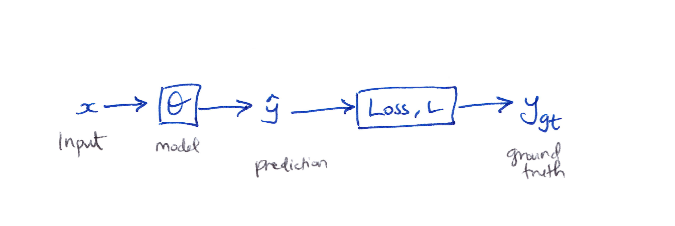
Gradient Descent
Gradient descent updates the model parameters by stepping in the direction that reduces the loss, using the gradient as a guide for how to adjust each parameter. The momentum and velocity terms refine this process by smoothing past gradients and scaling updates adaptively, which helps stabilize training and converge faster, especially in noisy or complex loss landscapes.
\[\begin{aligned} \text{simply} \quad & \Theta_i \leftarrow \Theta_{i-1} - \alpha \frac{\partial L}{\partial \Theta_i} \\[6pt] \text{momentum} \quad & M_i \leftarrow \beta_1 M_{i-1} + (1 - \beta_1) \frac{\partial L}{\partial \Theta_i} \\[6pt] \text{velocity} \quad & V_i \leftarrow \beta_2 V_{i-1} + (1 - \beta_2) \left(\frac{\partial L}{\partial \Theta_i}\right)^2 \\[6pt] & \Theta_i \leftarrow \Theta_{i-1} - \alpha \left(\frac{M_i}{\sqrt{V_i} + \varepsilon}\right) \end{aligned}\] \[\begin{aligned} \text{where} \\ M_i &\equiv \text{momentum (1st moment)} \\ V_i &\equiv \text{velocity: gradient squared (2nd moment)} \\ \beta_1, \beta_2 &\equiv \text{decay hyperparameters} \\ \varepsilon &\equiv \text{small constant for numerical stability} \end{aligned}\]Cons of Adam
- Memory intensive.
- Challenging hyper-parameter tuning.
- Independent update of each value in a single, long, parameter vector without considering any internal structure (vector-based optimizer behavior) of the model parameters.3
Question: Can we explicitly account for the underlying matrix structure of the model parameters?
The Linear Layer & Matrix Momentum
-
For a linear layer with 3 inputs $(x_1, x_2, x_3)$ and 4 outputs $(z_1, z_2, z_3, z_4)$:
\[z_i = \Theta_{i1} x_1 + \Theta_{i2} x_2 + \Theta_{i3} x_3, \quad \forall\, i = 1, 2, 3, 4\]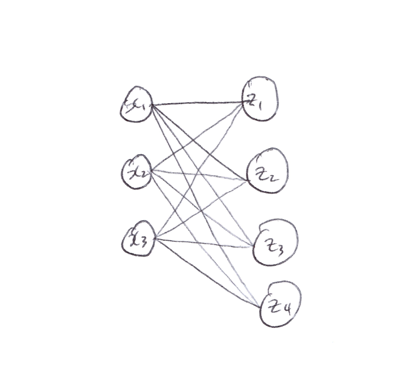
-
In matrix form:
\[\begin{bmatrix} z_1 \\ z_2 \\ z_3 \\ z_4 \end{bmatrix} = \begin{bmatrix} \Theta_{11} & \Theta_{12} & \Theta_{13} \\ \Theta_{21} & \Theta_{22} & \Theta_{23} \\ \Theta_{31} & \Theta_{32} & \Theta_{33} \\ \Theta_{41} & \Theta_{42} & \Theta_{43} \end{bmatrix} \begin{bmatrix} x_1 \\ x_2 \\ x_3 \end{bmatrix}\] -
Since $\Theta$ is now a matrix, we need a matrix momentum $\hat{M}$ for $\hat{\Theta}$:
\[\hat{M} = \begin{bmatrix} m_{11} & m_{12} & m_{13} \\ m_{21} & m_{22} & m_{23} \\ m_{31} & m_{32} & m_{33} \\ m_{41} & m_{42} & m_{43} \end{bmatrix}\] -
So the matrix momentum update is:
\[\hat{M}_i \leftarrow \beta \hat{M}_i + \frac{\partial L}{\partial \hat{\Theta}_i}\]
The Problem with Vector-Based Optimizers
- With vector-based optimizers like Adam, the momentum for a linear layer (a 2D matrix) tends to become almost low rank in practice.
- Essentially, only a small number of dominant directions really drive the update, while the many remaining other directions contribute very little.
Question: How can we tackle this update direction imbalance and what makes a good optimizer?
From fundamental first principles, a good optimizer possesses two characteristics: stability and speed. The goal of each update of a good optimizer is to minimize model variance and maximize loss reduction contribution, which correspond to stability and speed respectively.1
Matrix Orthogonalization
- We can fix the imbalance of update directions via orthogonalization.
- Orthogonalize the momentum matrix. This is where Muon comes in.
- It amplifies the effect of rare directions – the directions that typically receive small or infrequent updates.
- Even though these rare directions seem minor, they are often essential for effective learning and can help capture more nuance patterns in the data.
Orthogonalization via SVD
-
We want the orthogonal matrix $O$ closest to $M$:
\[\text{Ortho}(M) = \arg\min_{O} \left\{\| O - M \|_F\right\} \quad \text{subject to } OO^T = I \text{ or } O^TO = I\] -
Using SVD (Singular Value Decomposition): $M = USV^T$, where:
\[\begin{aligned} UU^T &= U^TU = I \\ VV^T &= V^TV = I \end{aligned} \quad \bigg\} \text{ orthonormal matrices}\] -
Since $OO^T = O^TO = I$:
\[\therefore\quad O = USV^T \quad \text{where } S = \begin{bmatrix} 1 & & 0 \\ & \ddots & \\ 0 & & 1 \end{bmatrix} \equiv \text{unit diagonal matrix}\] -
Issue: SVD on a matrix is computationally expensive.
-
Fix: Use an odd polynomial matrix:
\[p(X) = aX + b(XX^T)X\]
Odd Polynomial Matrix
\[\begin{align*} p(M) &= a(M) + b(MM^T)M \\ &= \left(aI + b(MM^T)\right)M \\ &= \left(aI + b(USV^T VS U^T)\right)USV^T \\ &= \left(aI + b(US^2 U^T)\right)USV^T \\ &= aUSV^T + bUS^2 U^T USV^T \\ p(M) &= aUSV^T + bUS^3V^T \\ \end{align*}\]-
This applies to any odd polynomial, so in general:
\[p(M) = U\!\left(aS + bS^3 + cS^5 + \ldots + (\text{const})\, S^{2n+1}\right)V^T, \quad \forall\, n \geq 0,\ n \to \infty\] -
Sticking to the 5th order polynomial:
\[\boxed{p(M) = U\!\left(aS + bS^3 + cS^5\right)V^T}\] -
We need to determine the coefficients $(a, b, c)$. The goal is to get $S$ to a unit diagonal matrix – i.e., get the diagonal values as close to 1 as possible.
-
Example: Plot $y = p(x)$ against $x$. If $(a, b, c) = (1.5,\ -0.5,\ 0)$:
\[y = 1.5x - 0.5x^3\]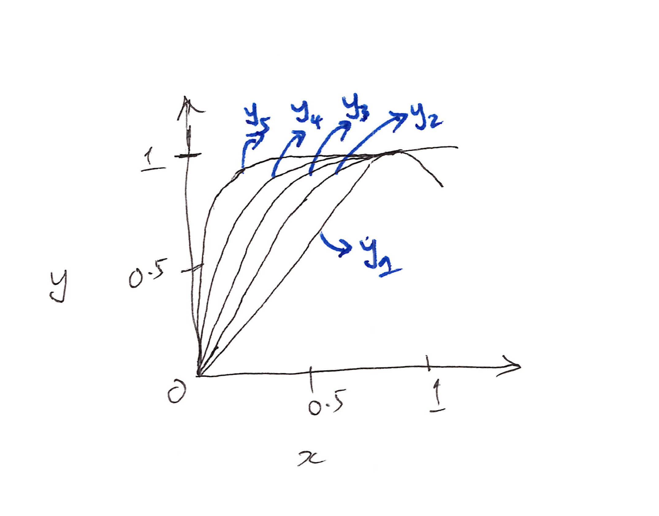
-
Applying this repeatedly via Newton-Schulz iteration:
- Each $y_k$ represents one more composition: $y_1 \to y_5$ are multiple iterations aimed at converging the singular values toward 1.
Newton-Schulz-5 Iteration
- After 5 iterations, almost all input values end up very close to 1.
- We can change $(a, b, c)$ to see the effect on convergence of $y$ to 1.
-
$(a, b, c) = (2,\ -1.5,\ 0.5)$ speeds up the convergence to 1.
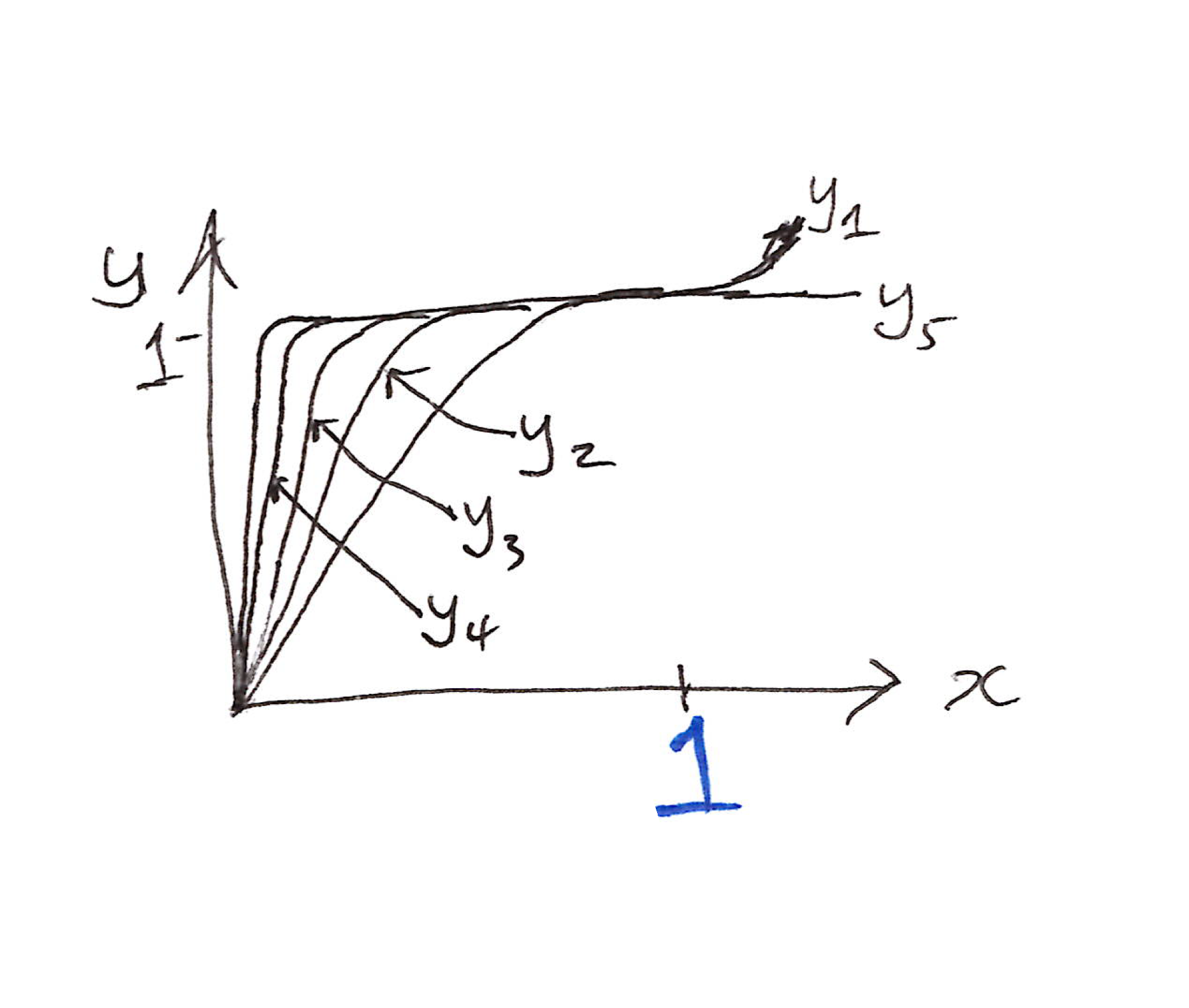
- Empirically, we don’t need the singular values to converge to exactly 1.
- Let’s set an upper & lower bound, e.g. $(0.7,\ 1.3)$, which is basically $[1 - \varepsilon, 1 + \varepsilon]$.
-
Tuned coefficients:
\[\boxed{(a,\ b,\ c) = (3.4445,\ -4.775,\ 2.0315)}\] -
Each Newton-Schulz 5 iteration involves only matrix multiplication:
\[X \leftarrow aX + b(XX^T)X + c(XX^T)^2 X\] - With GPUs, no need to use SVD since GPUs can efficiently compute matrix multiplication.
def newtonschulz5(G, steps=5, eps=1e-7):
    assert G.ndim == 2
    a, b, c = (3.4445, -4.7750, 2.0315)
    X = G.bfloat16()
    X /= (X.norm() + eps)
    if G.size(0) > G.size(1):
        X = X.T
    for _ in range(steps):
        A = X @ X.T
        B = b * A + c * A @ A
        X = a * X + B @ X
    if G.size(0) > G.size(1):
        X = X.T
    return X

# Retrieved from https://kellerjordan.github.io/posts/muon/
Muon
Muon is designed specifically for 2D weight matrices in neural network hidden layers.4 Unlike traditional optimizers that treat each parameter independently, Muon leverages the geometric structure of weight matrices by orthogonalizing gradients using the Newton-Schulz iteration. Muon is specifically designed for linear neural network layers, which aligns with ongoing research that argues that different layer types require different optimizers due to their varying geometry.5
The optimizer formulates weight updates as a constrained optimization problem in the RMS-to-RMS operator norm space:
\[\text{Ortho}(M) = \arg\min_{O} \left\{\| O - M \|_F\right\} \quad \text{subject to } OO^T = I \text{ or } O^TO = I\]Where $M$ is the gradient matrix. The solution involves projecting the gradient onto the set of orthogonal matrices, which aims to standardize all singular values to 1 while preserving gradient directions.
Pseudo-Algorithm for Muon
for t = 1, 2, ..., do:
    Compute gradient      G_t  ←  ∇L_t(θ_{t-1})
    Compute momentum      M_t  ←  βM_{t-1} + G_t
    Normalize             M'_t ←  M_t / ||M_t||_F
    Orthogonalization     O_t  ←  NewtonSchutz5(M'_t)
    Update parameter      θ_t  ←  θ_{t-1} - α O_t
-
With weight decay $(+)$:
\[\Theta_t \leftarrow \Theta_{t-1} - \alpha\!\left(O_t + \lambda\Theta_{t-1}\right)\] -
With adjusted learning rate $(+)$:
\[\Theta_t \leftarrow \Theta_{t-1} - \alpha\!\left[\left(0.2\sqrt{\max(n,m)}\right) O_t + \lambda\Theta_{t-1}\right]\] \[\begin{aligned} \text{where} \\ \lambda &\equiv \text{weight decay coefficient} \\ n, m &\equiv \text{dimensions of the 2D parameter matrix} \end{aligned}\]
Muon + Weight Decay + RMS Alignment
- Weight decay is used to address the diminished performance gains of Muon over AdamW when scaling up to train a larger model.
- The learning rate also gets adjusted by taking into account the size of the 2D matrix. This is the underlying principle behind the RMS (Root Mean Squared) Alignment.
- The scaling factor used to scale the Muon update for each matrix to ensure per-matrix parameter update RMS alignment of around 1 of matrices of different shapes is $\sqrt(\max(A, B))$ for a full-rank weight matrix of shape $[A,\ B]$.6
- The $0.2$ factor is used to match Muon’s update RMS to that of AdamW. From empirical observations, AdamW’s update RMS is usually around $0.2$ to $0.4$.6, 1
- These 2 improvements (weight decay & adjusting the per-parameter update scale) help to stabilize the training of large models.
The Exploding Attention Logit Crisis
- Issue: Attention logits can grow larger & larger as training continues, which may cause the training process to become unstable.
-
Consider a sequence of 4 tokens & assume self-attention for simplicity. Each token is mapped to an embedding vector of dimension $d$. Let the embedding matrix be $X$.
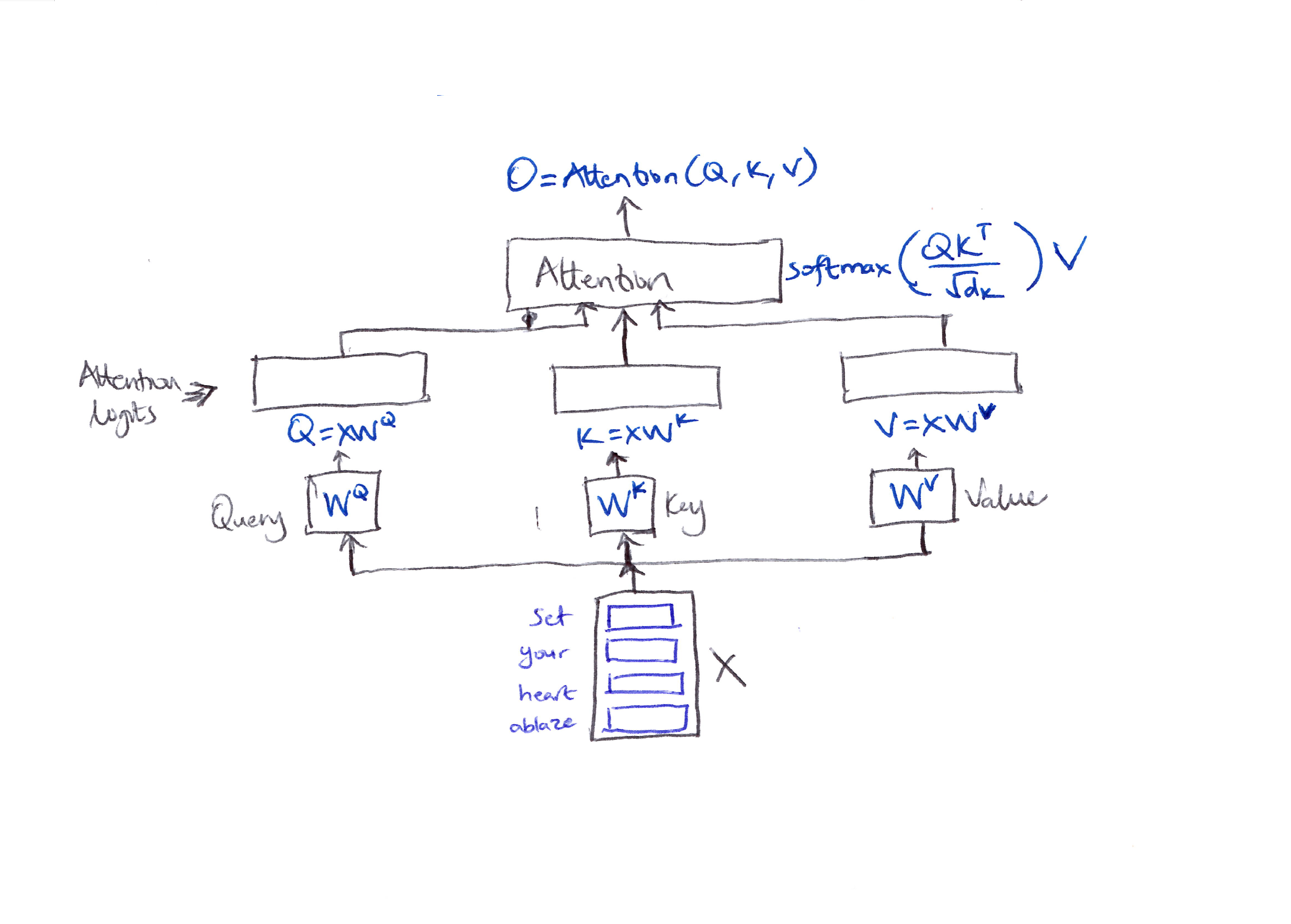
$O = \text{Attention}(Q, K, V) = \text{softmax}\left(\frac{QK^T}{\sqrt{d_k}}\right)V$
- In self attention above, $Q = XW^Q$, $K = XW^K$, and $V = XW^V$.
-
The attention logits $S$:
\[\begin{align*} S &= QK^T \\ &= (XW^Q)(XW^K)^T \\ &= X\!\left(W^Q W^{K^T}\right)X^T \end{align*}\]where $X$ and $X^T$ denote the embedding vectors, which are typically normalized to have unit norms.
-
To prevent the attention logits from becoming excessively large, we must control the scale of $W^Q$ and $W^K$:
\[S = X\underbrace{\left(W^Q W^{K^T}\right)}_{\text{scale control}}X^T\]
QK-Clip
- A common strategy is to apply a scaling vector to these matrices.
- During training, monitor the maximum value of the attention logits, $S_{\max}$. If it exceeds a certain threshold $\tau$, calculate a scaling ratio $\gamma$:
- Directly constrains attention logits, ensuring they stay within a safe range by rescaling the query & key projection weights.
Idea: Scale the relevant model parameters by $\gamma$ when the attention logits surpass the threshold. Scale both $W^Q$, $W^K$ by $\sqrt{\gamma}$:
\[\begin{align*} S &= X\!\left(\gamma W^Q W^{K^T}\right)X^T \\ &= X\!\left(\sqrt{\gamma}\, W^Q\ \sqrt{\gamma}\, W^{K^T}\right)X^T \end{align*}\]Revised pseudo-algorithm (QK-Clip):
θ_t ← MuonOptimizer(θ_{t-1}, G_t)
if S_max > τ:
    W^Q ← √γ W^Q
    W^K ← √γ W^K
QK-Clip for Multi-Head Attention
- In practice, self-attention consists of multiple heads ($n_{\text{heads}} = h$).
-
When the maximum attention logits exceed the threshold, instead of rescaling all heads in the same way (which doesn’t make sense), we introduce an individual scaling factor for each head to control their logits separately.
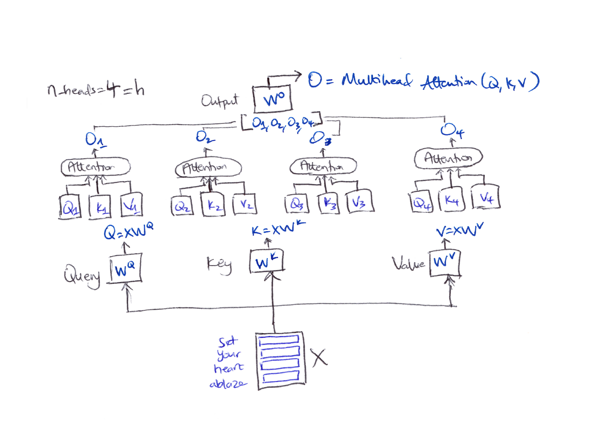
$O = \text{MultiheadAttention}(Q, K, V) = \text{Concat}(head_0, head_1, .., head_h) W_o$
-
Attention logits per head:
\[S = X\!\left(\sqrt{\gamma_h}\, W_h^Q\ \sqrt{\gamma_h}\, W_h^{K^T}\right)X^T\] \[\text{if } S_{\max}^h > \tau \quad \text{then} \quad \gamma_h = \frac{\tau}{S_{\max}}\]
Algorithm for Muon + QK-Clip for MHA:
θ_t ← MuonOptimizer(θ_{t-1}, G_t)
if S^h_max > τ:
    W^Q_h ← √γ_h W^Q_h
    W^K_h ← √γ_h W^K_h
Multihead Latent Attention (MLA)
-
For multihead Latent Attention (MLA) by DeepSeek, things get tricky.
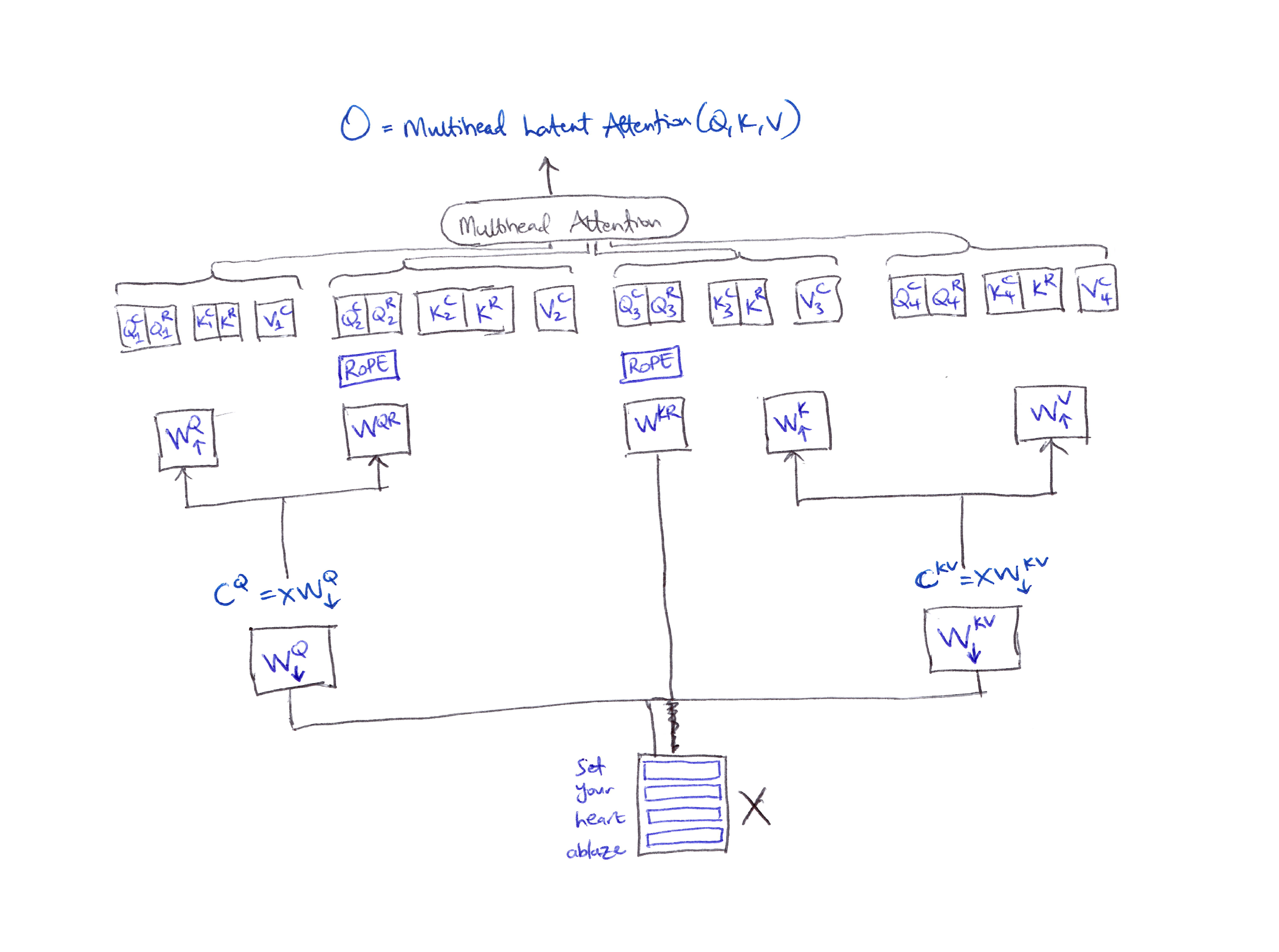
-
MLA compresses $Q, K, V$ representations into a low-rank space to reduce the size of the KV cache using a down-projection matrix which produces latent representations:
\[C^Q = XW^Q_\downarrow \qquad C^{KV} = XW^{KV}_\downarrow\] - These compressed latent vectors are then mapped back to $W^Q_\uparrow$, $W^K_\uparrow$, $W^V_\uparrow$ for each attention head using the corresponding up-projection matrices.
- Issue: This low-rank KV compression fails with rotary position embedding (RoPE).
- Fix: A decoupled RoPE technique which introduces extra multi-head queries $W^{QR}$ and a shared key $W^{KR}$ to encode positional information.
- For MLA, the Query, Key & Values are regrouped for each head:
- The Query is constructed by concatenating the compressed query $Q^C$ with the rotated query $Q^R$.
- The Key is constructed similarly by concatenating the compressed key $K^C$ with the rotated key $K^R$.
MLA compresses $Q, K, V$ representations into a low-rank latent space via down-projection matrices $W^Q_\downarrow$ and $W^{KV}_\downarrow$, then maps back up via up-projection matrices. A decoupled RoPE technique adds rotary queries $W^{QR}$ and a shared rotary key $W^{KR}$.
MuonClip
In MLA, it is important to carefully decide how to rescale these 4 matrices: $W^Q_\uparrow,\ W^{QR},\ W^{KR},\ W^K_\uparrow$.
- For the up-projection matrices $W^Q_\uparrow$, $W^K_\uparrow$: rescale these parameters for each head individually.
- The RoPE components $W^{QR}$, $W^{KR}$ rescaling is more tricky:
- Each head has its own rotary query $W^{QR}$.
- But all heads share a single rotary key matrix $W^{KR}$.
Issue: Applying the same per-head scaling for both RoPE components leads to the shared $W^{KR}$ being rescaled multiple times, which is undesirable.
Fix: Rescale only the head-specific rotary query $W^{QR}$ by their respective $\gamma^h$, while leaving the shared rotary key matrix $W^{KR}$ unchanged. This technique is called MuonClip. MuonClip improves upon Muon with the QK-Clip technique to handle training instability while benefiting from Muon’s advanced token efficiency.7
MuonClip Algorithm:
θ_t ← MuonOptimizer(θ_{t-1}, G_t)
if S^h_max > τ:
    γ_h = τ / S^h_max
    W^Q_{h,↑}  ← √γ_h  W^Q_{h,↑}
    W^K_{h,↑}  ← √γ_h  W^K_{h,↑}
    W^{QR}_h   ← γ_h   W^{QR}_h
    W^{KR}     ← W^{KR}   (unchanged)
In math:
\[\begin{aligned} \gamma_h &= \frac{\tau}{S_{\max}^h} \\[6pt] W_{h,\uparrow}^Q &\leftarrow \sqrt{\gamma_h}\, W_{h,\uparrow}^Q \\ W_{h,\uparrow}^K &\leftarrow \sqrt{\gamma_h}\, W_{h,\uparrow}^K \\ W_h^{QR} &\leftarrow \gamma_h\, W_h^{QR} \\ W^{KR} &\leftarrow W^{KR} \quad \text{(unchanged)} \end{aligned}\]Citation
If you found this blog post helpful, please consider citing it:
@article{obasi2026muonmuonclip,
  title   = "Muon & MuonClip Optimizers",
  author  = "Obasi, Chizoba",
  journal = "chizkidd.github.io",
  year    = "2026",
  month   = "Apr",
  url     = "https://chizkidd.github.io/2026/04/04/muon-muonclip/"
}
References
-
Kimi (Moonshot AI). Why We Chose Muon: Our Chain of Thought. X (Twitter). 2025. ↩ ↩2 ↩3
-
Chizoba Obasi. A Complete Guide to Neural Network Optimizers. chizkidd.github.io. 2026. ↩
-
Jia-Bin Huang This Simple Optimizer Is Revolutionizing How We Train AI [Muon] (YouTube Video). YouTube. ↩
-
Keller Jordan. Muon: An optimizer for hidden layers in neural networks. kellerjordan.github.io. 2024. ↩
-
Jeremy Bernstein. Deriving Muon. jeremybernste.in. 2025. ↩
-
Muon is Scalable for LLM Training. arXiv. 2025. ↩ ↩2
-
Kimi K2: Open Agentic Intelligence. arXiv. 2025. ↩