Deep Learning Models: A collection of various deep learning architectures, models, & their implementations (PyTorch or TensorFlow) in Jupyter Notebooks.
- Author: Chizoba Obasi
- Github Repo: https://github.com/chizkidd/deep-learning-models
!pip install watermark
Collecting watermark
  Downloading watermark-2.6.0-py3-none-any.whl.metadata (15 kB)
Requirement already satisfied: ipython>=6.0 in /usr/local/lib/python3.12/dist-packages (from watermark) (7.34.0)
Requirement already satisfied: importlib-metadata>=1.4 in /usr/local/lib/python3.12/dist-packages (from watermark) (8.7.0)
Requirement already satisfied: setuptools in /usr/local/lib/python3.12/dist-packages (from watermark) (75.2.0)
Requirement already satisfied: zipp>=3.20 in /usr/local/lib/python3.12/dist-packages (from importlib-metadata>=1.4->watermark) (3.23.0)
Requirement already satisfied: jedi>=0.16 in /usr/local/lib/python3.12/dist-packages (from ipython>=6.0->watermark) (0.19.2)
Requirement already satisfied: decorator in /usr/local/lib/python3.12/dist-packages (from ipython>=6.0->watermark) (4.4.2)
Requirement already satisfied: pickleshare in /usr/local/lib/python3.12/dist-packages (from ipython>=6.0->watermark) (0.7.5)
Requirement already satisfied: traitlets>=4.2 in /usr/local/lib/python3.12/dist-packages (from ipython>=6.0->watermark) (5.7.1)
Requirement already satisfied: prompt-toolkit!=3.0.0,!=3.0.1,<3.1.0,>=2.0.0 in /usr/local/lib/python3.12/dist-packages (from ipython>=6.0->watermark) (3.0.52)
Requirement already satisfied: pygments in /usr/local/lib/python3.12/dist-packages (from ipython>=6.0->watermark) (2.19.2)
Requirement already satisfied: backcall in /usr/local/lib/python3.12/dist-packages (from ipython>=6.0->watermark) (0.2.0)
Requirement already satisfied: matplotlib-inline in /usr/local/lib/python3.12/dist-packages (from ipython>=6.0->watermark) (0.1.7)
Requirement already satisfied: pexpect>4.3 in /usr/local/lib/python3.12/dist-packages (from ipython>=6.0->watermark) (4.9.0)
Requirement already satisfied: parso<0.9.0,>=0.8.4 in /usr/local/lib/python3.12/dist-packages (from jedi>=0.16->ipython>=6.0->watermark) (0.8.5)
Requirement already satisfied: ptyprocess>=0.5 in /usr/local/lib/python3.12/dist-packages (from pexpect>4.3->ipython>=6.0->watermark) (0.7.0)
Requirement already satisfied: wcwidth in /usr/local/lib/python3.12/dist-packages (from prompt-toolkit!=3.0.0,!=3.0.1,<3.1.0,>=2.0.0->ipython>=6.0->watermark) (0.2.14)
Downloading watermark-2.6.0-py3-none-any.whl (13 kB)
Installing collected packages: watermark
Successfully installed watermark-2.6.0
!pip install torchinfo
Requirement already satisfied: torchinfo in /usr/local/lib/python3.12/dist-packages (1.8.0)
%load_ext watermark
# %reload_ext watermark
%watermark -a 'Chizoba Obasi' -v -p torch
Author: Chizoba Obasi

Python implementation: CPython
Python version       : 3.12.12
IPython version      : 7.34.0

torch: 2.8.0+cu126
MobileNetV2 Classifier on CIFAR-10
This notebook implements MobileNetV2 [1] and applies it to the CIFAR-10 dataset.
Network Architecture
MobileNetV1 Core Idea: Depthwise Separable Convolutions
In a standard convolution, the filter tries to learn both spatial (height/width) and cross-channel (depth) features simultaneously. Depthwise separable convolution breaks this down into two distinct steps:
- Depthwise (DW) Convolution:
- A spatial convolution is performed independently on each input channel.
CONV(3x3 DW)->BatchNORM->ReLU
- Pointwise (PW) Convolution:
- A convolution is then applied to project the channels into a new space.
CONV(1x1)->BatchNORM->ReLU
Standard Convolution ($L$) vs Depthwise Separable Convolutions ($R$)

MobileNetV2: Core Idea

Non-Linearity Implementation: ReLU6

Core Breakthrough: Inverted Residual & Linear Bottleneck

To build MobileNetV2 from scratch for CIFAR-10, we need to implement its defining feature: the Inverted Residual Block.
Unlike standard ResNet blocks that go "wide->narrow->wide" (bottleneck), MobileNetV2 goes "narrow ->wide ->narrow". This allows the network to process more detailed features in the expanded high-dimensional space while keeping the connections between blocks "thin" to save memory.
1. The Inverted Residual Block
This block consists of three layers:
- Expansion: A convolution that increases the number of channels.
- Depthwise: A depthwise convolution to filter the features.
- Projection (Linear Bottleneck): A convolution that shrinks the channels back down. Crucially, this layer has no activation function to prevent information loss.
REFERENCES:
- Sandler, M., et al. "MobileNetV2: Inverted Residuals and Linear Bottlenecks " CVPR, 2018.
- Johnson, J. (2022, February 2). Lecture 11: CNN Architectures, Part 2 [PowerPoint Slides]. University of Michigan EECS 498/598: Deep Learning for Computer Vision. pp 44-53. https://web.eecs.umich.edu/~justincj/slides/eecs498/WI2022/598_WI2022_lecture11.pdf
import torch
import torchvision
import torch.nn as nn
import torch.nn.functional as F
import torch.optim as optim
from torch.utils.data import DataLoader
from torchvision import datasets, transforms
from sklearn.model_selection import train_test_split

from torchinfo import summary

import matplotlib.image as mpimg
import matplotlib.pyplot as plt
%matplotlib inline

import pandas as pd
import numpy as np
import math
import time
import os
import random

if torch.cuda.is_available():
    torch.backends.cudnn.deterministic = True
def set_all_seeds(seed):
    os.environ["PL_GLOBAL_SEED"] = str(seed)
    random.seed(seed)
    np.random.seed(seed)
    torch.manual_seed(seed)
    torch.cuda.manual_seed_all(seed)
# Check if GPU is available and set the device
if torch.cuda.is_available():
    num_gpus = torch.cuda.device_count()
    print("Num GPUs Available: ", num_gpus)
    for i in range(num_gpus):
        gpu_name = torch.cuda.get_device_name(i)
        print(f"GPU {i}: {gpu_name}")
else:
    print("No GPU available.")
Num GPUs Available:  2
GPU 0: Tesla T4
GPU 1: Tesla T4
##########################
### SETTINGS
##########################

# Hyperparameters
RANDOM_SEED = 123
BATCH_SIZE = 128 #256
LEARNING_RATE = 0.001
NUM_EPOCHS = 50 #30
INPUT_SIZE = 32 # CIFAR-10 is 32x32
NUM_CLASSES = 10

# Set device
device = torch.device("cuda" if torch.cuda.is_available() else "cpu")
print(device)
cuda
set_all_seeds(RANDOM_SEED)
1. Data Preparation & Loading
Notes:
- Since we adjust the model to handle the CIFAR images natively, we should remove the
Resize((xx, yy))from your transforms. It will make ythe training 10x faster and use significantly less memory.
# CIFAR-10 specific stats (MEAN_arr, STD_arr)
stats = ((0.4914, 0.4822, 0.4465), (0.2471, 0.2435, 0.2616)) #(0.2023, 0.1994, 0.2010))

train_transforms = transforms.Compose([
    transforms.RandomCrop(32, padding=4), # Standard CIFAR augmentation
    transforms.RandomHorizontalFlip(),
    transforms.ToTensor(),
    transforms.Normalize(*stats)
])

test_transforms = transforms.Compose([
    transforms.ToTensor(),
    transforms.Normalize(*stats)
])

# Load Datasets
train_dataset = datasets.CIFAR10(root='./data', train=True, download=True, transform=train_transforms)
test_dataset = datasets.CIFAR10(root='./data', train=False, download=True, transform=test_transforms)

# Split training set into training and validation sets
train_size = int(0.9 * len(train_dataset))
val_size = len(train_dataset) - train_size
train_subset, val_subset = torch.utils.data.random_split(train_dataset, [train_size, val_size])

# Create DataLoaders
train_loader = DataLoader(train_subset, batch_size=BATCH_SIZE, shuffle=True, num_workers=2, pin_memory=True)
val_loader = DataLoader(val_subset, batch_size=BATCH_SIZE, shuffle=False, num_workers=2, pin_memory=True)
test_loader = DataLoader(test_dataset, batch_size=BATCH_SIZE, shuffle=False, num_workers=2, pin_memory=True)

classes = ('plane', 'car', 'bird', 'cat', 'deer', 'dog', 'frog', 'horse', 'ship', 'truck')
100%|██████████| 170M/170M [00:03<00:00, 51.6MB/s]
# Checking the dataset
for images, labels in train_loader:
    print('Image batch dimensions:', images.shape)
    print('Image label dimensions:', labels.shape)
    print('Class labels of 10 examples:', labels[:10])
    break
Image batch dimensions: torch.Size([128, 3, 32, 32])
Image label dimensions: torch.Size([128])
Class labels of 10 examples: tensor([2, 7, 4, 7, 0, 1, 1, 6, 9, 2])
plt.figure(figsize=(8, 8))
plt.axis("off")
plt.title("Training Images")
plt.imshow(np.transpose(torchvision.utils.make_grid(images[:64],
                                         padding=2, normalize=True),
                        (1, 2, 0)))
<matplotlib.image.AxesImage at 0x7c16a6943fb0>

2. Model Creation
Notes:
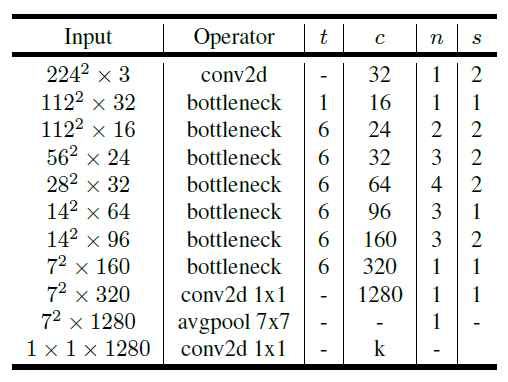
- For CIFAR-10, we modify the original architecture by setting the initial convolution stride to 1 instead of 2. This prevents the $32 \times 32$ image from shrinking too fast.
class InvertedResidual(nn.Module):
    def __init__(self, in_channels, out_channels, stride, expand_ratio):
        super(InvertedResidual, self).__init__()
        self.stride = stride
        hidden_dim = int(in_channels * expand_ratio)

        # Shortcut is only used if input/output shapes match and stride is 1
        self.use_res_connect = self.stride == 1 and in_channels == out_channels

        layers = []
        if expand_ratio != 1:
            # 1. Expansion (1x1)
            layers.append(nn.Conv2d(in_channels, hidden_dim, 1, 1, 0, bias=False))
            layers.append(nn.BatchNorm2d(hidden_dim))
            layers.append(nn.ReLU6(inplace=True))

        layers.extend([
            # 2. Depthwise (3x3)
            nn.Conv2d(hidden_dim, hidden_dim, 3, stride, 1, groups=hidden_dim, bias=False),
            nn.BatchNorm2d(hidden_dim),
            nn.ReLU6(inplace=True),
            # 3. Projection (1x1) - Note: No ReLU here (Linear Bottleneck)
            nn.Conv2d(hidden_dim, out_channels, 1, 1, 0, bias=False),
            nn.BatchNorm2d(out_channels),
        ])

        self.conv = nn.Sequential(*layers)

    def forward(self, x):
        if self.use_res_connect:
            return x + self.conv(x)
        else:
            return self.conv(x)


class MobileNetV2(nn.Module):
    def __init__(self, num_classes=10):
        super(MobileNetV2, self).__init__()

        # (expansion_factor t, output_channels c, num_blocks n, stride s)
        self.configs = [
            [1, 16, 1, 1],
            [6, 24, 2, 1], # Stride 1 for CIFAR
            [6, 32, 3, 2],
            [6, 64, 4, 2],
            [6, 96, 3, 1],
            [6, 160, 3, 2],
            [6, 320, 1, 1],
        ]

        # Initial Layer: Conv3x3 Stride 1 for CIFAR
        self.first_conv = nn.Sequential(
            nn.Conv2d(3, 32, 3, 1, 1, bias=False),
            nn.BatchNorm2d(32),
            nn.ReLU6(inplace=True)
        )

        # Build Inverted Residual Blocks
        layers = []
        input_channel = 32
        for t, c, n, s in self.configs:
            for i in range(n):
                stride = s if i == 0 else 1
                layers.append(InvertedResidual(input_channel, c, stride, expand_ratio=t))
                input_channel = c
        self.blocks = nn.Sequential(*layers)

        # Final Layers
        self.last_conv = nn.Sequential(
            nn.Conv2d(input_channel, 1280, 1, 1, 0, bias=False),
            nn.BatchNorm2d(1280),
            nn.ReLU6(inplace=True)
        )

        self.classifier = nn.Sequential(
            nn.Dropout(0.2),
            nn.Linear(1280, num_classes)
        )

    def forward(self, x):
        x = self.first_conv(x)
        x = self.blocks(x)
        x = self.last_conv(x)
        x = x.mean([2, 3]) # Global Average Pooling
        x = self.classifier(x)
        return x
model = MobileNetV2().to(device)
# Model parameter details
summary(model,
        input_size=(BATCH_SIZE, 3, INPUT_SIZE, INPUT_SIZE),
        # verbose=1,
        col_names=["input_size", "output_size", "num_params", "kernel_size", "mult_adds"]
       )
=====================================================================================================================================================================
Layer (type:depth-idx)                   Input Shape               Output Shape              Param #                   Kernel Shape              Mult-Adds
=====================================================================================================================================================================
MobileNetV2                              [128, 3, 32, 32]          [128, 10]                 --                        --                        --
├─Sequential: 1-1                        [128, 3, 32, 32]          [128, 32, 32, 32]         --                        --                        --
│    └─Conv2d: 2-1                       [128, 3, 32, 32]          [128, 32, 32, 32]         864                       [3, 3]                    113,246,208
│    └─BatchNorm2d: 2-2                  [128, 32, 32, 32]         [128, 32, 32, 32]         64                        --                        8,192
│    └─ReLU6: 2-3                        [128, 32, 32, 32]         [128, 32, 32, 32]         --                        --                        --
├─Sequential: 1-2                        [128, 32, 32, 32]         [128, 320, 4, 4]          --                        --                        --
│    └─InvertedResidual: 2-4             [128, 32, 32, 32]         [128, 16, 32, 32]         --                        --                        --
│    │    └─Sequential: 3-1              [128, 32, 32, 32]         [128, 16, 32, 32]         896                       --                        104,869,888
│    └─InvertedResidual: 2-5             [128, 16, 32, 32]         [128, 24, 32, 32]         --                        --                        --
│    │    └─Sequential: 3-2              [128, 16, 32, 32]         [128, 24, 32, 32]         5,136                     --                        616,617,984
│    └─InvertedResidual: 2-6             [128, 24, 32, 32]         [128, 24, 32, 32]         --                        --                        --
│    │    └─Sequential: 3-3              [128, 24, 32, 32]         [128, 24, 32, 32]         8,832                     --                        1,075,918,848
│    └─InvertedResidual: 2-7             [128, 24, 32, 32]         [128, 32, 16, 16]         --                        --                        --
│    │    └─Sequential: 3-4              [128, 24, 32, 32]         [128, 32, 16, 16]         10,000                    --                        646,529,024
│    └─InvertedResidual: 2-8             [128, 32, 16, 16]         [128, 32, 16, 16]         --                        --                        --
│    │    └─Sequential: 3-5              [128, 32, 16, 16]         [128, 32, 16, 16]         14,848                    --                        459,382,784
│    └─InvertedResidual: 2-9             [128, 32, 16, 16]         [128, 32, 16, 16]         --                        --                        --
│    │    └─Sequential: 3-6              [128, 32, 16, 16]         [128, 32, 16, 16]         14,848                    --                        459,382,784
│    └─InvertedResidual: 2-10            [128, 32, 16, 16]         [128, 64, 8, 8]           --                        --                        --
│    │    └─Sequential: 3-7              [128, 32, 16, 16]         [128, 64, 8, 8]           21,056                    --                        316,260,352
│    └─InvertedResidual: 2-11            [128, 64, 8, 8]           [128, 64, 8, 8]           --                        --                        --
│    │    └─Sequential: 3-8              [128, 64, 8, 8]           [128, 64, 8, 8]           54,272                    --                        431,177,728
│    └─InvertedResidual: 2-12            [128, 64, 8, 8]           [128, 64, 8, 8]           --                        --                        --
│    │    └─Sequential: 3-9              [128, 64, 8, 8]           [128, 64, 8, 8]           54,272                    --                        431,177,728
│    └─InvertedResidual: 2-13            [128, 64, 8, 8]           [128, 64, 8, 8]           --                        --                        --
│    │    └─Sequential: 3-10             [128, 64, 8, 8]           [128, 64, 8, 8]           54,272                    --                        431,177,728
│    └─InvertedResidual: 2-14            [128, 64, 8, 8]           [128, 96, 8, 8]           --                        --                        --
│    │    └─Sequential: 3-11             [128, 64, 8, 8]           [128, 96, 8, 8]           66,624                    --                        531,849,216
│    └─InvertedResidual: 2-15            [128, 96, 8, 8]           [128, 96, 8, 8]           --                        --                        --
│    │    └─Sequential: 3-12             [128, 96, 8, 8]           [128, 96, 8, 8]           118,272                   --                        948,756,480
│    └─InvertedResidual: 2-16            [128, 96, 8, 8]           [128, 96, 8, 8]           --                        --                        --
│    │    └─Sequential: 3-13             [128, 96, 8, 8]           [128, 96, 8, 8]           118,272                   --                        948,756,480
│    └─InvertedResidual: 2-17            [128, 96, 8, 8]           [128, 160, 4, 4]          --                        --                        --
│    │    └─Sequential: 3-14             [128, 96, 8, 8]           [128, 160, 4, 4]          155,264                   --                        652,681,216
│    └─InvertedResidual: 2-18            [128, 160, 4, 4]          [128, 160, 4, 4]          --                        --                        --
│    │    └─Sequential: 3-15             [128, 160, 4, 4]          [128, 160, 4, 4]          320,000                   --                        647,372,800
│    └─InvertedResidual: 2-19            [128, 160, 4, 4]          [128, 160, 4, 4]          --                        --                        --
│    │    └─Sequential: 3-16             [128, 160, 4, 4]          [128, 160, 4, 4]          320,000                   --                        647,372,800
│    └─InvertedResidual: 2-20            [128, 160, 4, 4]          [128, 320, 4, 4]          --                        --                        --
│    │    └─Sequential: 3-17             [128, 160, 4, 4]          [128, 320, 4, 4]          473,920                   --                        961,986,560
├─Sequential: 1-3                        [128, 320, 4, 4]          [128, 1280, 4, 4]         --                        --                        --
│    └─Conv2d: 2-21                      [128, 320, 4, 4]          [128, 1280, 4, 4]         409,600                   [1, 1]                    838,860,800
│    └─BatchNorm2d: 2-22                 [128, 1280, 4, 4]         [128, 1280, 4, 4]         2,560                     --                        327,680
│    └─ReLU6: 2-23                       [128, 1280, 4, 4]         [128, 1280, 4, 4]         --                        --                        --
├─Sequential: 1-4                        [128, 1280]               [128, 10]                 --                        --                        --
│    └─Dropout: 2-24                     [128, 1280]               [128, 1280]               --                        --                        --
│    └─Linear: 2-25                      [128, 1280]               [128, 10]                 12,810                    --                        1,639,680
=====================================================================================================================================================================
Total params: 2,236,682
Trainable params: 2,236,682
Non-trainable params: 0
Total mult-adds (Units.GIGABYTES): 11.27
=====================================================================================================================================================================
Input size (MB): 1.57
Forward/backward pass size (MB): 3358.60
Params size (MB): 8.95
Estimated Total Size (MB): 3369.12
=====================================================================================================================================================================
criterion = nn.CrossEntropyLoss()
optimizer = optim.Adam(model.parameters(), lr=LEARNING_RATE, weight_decay=5e-4)
# optimizer = optim.SGD(model.parameters(), lr=LEARNING_RATE, momentum=0.9, weight_decay=5e-4) # Use weight decay (L2) to combat overfitting
# scheduler = optim.lr_scheduler.ReduceLROnPlateau(optimizer, mode='min', factor=0.1, patience=5)

def calculate_accuracy(loader):
    model.eval()
    correct = 0
    total = 0
    with torch.no_grad():
        for inputs, labels in loader:
            inputs, labels = inputs.to(device), labels.to(device)
            outputs = model(inputs)
            _, predicted = torch.max(outputs.data, 1)
            total += labels.size(0)
            correct += (predicted == labels).sum().item()
    return 100 * correct / total

# Training Loop
start_time = time.time()
history = {'train_loss': [], 'val_loss': [], 'train_acc': [], 'val_acc': [], 'lrs': []}

print(f"Starting training on {device}...")

for epoch in range(NUM_EPOCHS):
    model.train()
    running_loss = 0.0

    for i, (inputs, labels) in enumerate(train_loader):
        inputs, labels = inputs.to(device), labels.to(device)

        optimizer.zero_grad()
        outputs = model(inputs)
        loss = criterion(outputs, labels)
        loss.backward()
        optimizer.step()

        running_loss += loss.item() * inputs.size(0)

    train_loss = running_loss / len(train_subset)
    train_acc = calculate_accuracy(train_loader)

    # Calculate validation loss and accuracy
    model.eval()
    val_loss = 0.0
    with torch.no_grad():
        for inputs, labels in val_loader:
            inputs, labels = inputs.to(device), labels.to(device)
            outputs = model(inputs)
            loss = criterion(outputs, labels)
            val_loss += loss.item() * inputs.size(0)

    val_loss /= len(val_subset)
    val_acc = calculate_accuracy(val_loader)

    # scheduler.step(val_loss)
    # current_lr = optimizer.param_groups[0]['lr']

    # Log metrics
    history['train_loss'].append(train_loss)
    history['val_loss'].append(val_loss)
    history['train_acc'].append(train_acc)
    history['val_acc'].append(val_acc)
    # history['lrs'].append(current_lr)

    print(f'Epoch {epoch + 1}/{NUM_EPOCHS} | '
          f'Train Loss: {train_loss:.5f}, '
          f'Train Acc.: {train_acc:.2f}% | '
          f'Val Loss: {val_loss:.5f}, '
          f'Val Acc.: {val_acc:.2f}% | '
          # f'LR: {current_lr:.8f}')
         )

print('\nTotal Training Time: %.2f min' % ((time.time() - start_time)/60))

# --- Final Evaluation ---
test_accuracy = calculate_accuracy(test_loader)
print(f'\nTest Accuracy: {test_accuracy:.2f}%')
Starting training on cuda...
Epoch 1/50 | Train Loss: 1.65259, Train Acc.: 44.32% | Val Loss: 1.62833, Val Acc.: 42.90% |
Epoch 2/50 | Train Loss: 1.24335, Train Acc.: 59.71% | Val Loss: 1.16926, Val Acc.: 57.62% |
Epoch 3/50 | Train Loss: 1.04269, Train Acc.: 67.01% | Val Loss: 1.02389, Val Acc.: 64.86% |
Epoch 4/50 | Train Loss: 0.90615, Train Acc.: 68.97% | Val Loss: 0.94685, Val Acc.: 67.12% |
Epoch 5/50 | Train Loss: 0.80052, Train Acc.: 73.14% | Val Loss: 0.83409, Val Acc.: 71.10% |
Epoch 6/50 | Train Loss: 0.72028, Train Acc.: 75.99% | Val Loss: 0.73896, Val Acc.: 73.86% |
Epoch 7/50 | Train Loss: 0.66346, Train Acc.: 78.86% | Val Loss: 0.67433, Val Acc.: 76.78% |
Epoch 8/50 | Train Loss: 0.61909, Train Acc.: 75.62% | Val Loss: 0.78513, Val Acc.: 73.10% |
Epoch 9/50 | Train Loss: 0.58585, Train Acc.: 80.78% | Val Loss: 0.65771, Val Acc.: 77.38% |
Epoch 10/50 | Train Loss: 0.55204, Train Acc.: 81.91% | Val Loss: 0.61914, Val Acc.: 78.92% |
Epoch 11/50 | Train Loss: 0.52964, Train Acc.: 82.52% | Val Loss: 0.57934, Val Acc.: 80.16% |
Epoch 12/50 | Train Loss: 0.50480, Train Acc.: 83.16% | Val Loss: 0.57475, Val Acc.: 79.78% |
Epoch 13/50 | Train Loss: 0.48471, Train Acc.: 82.10% | Val Loss: 0.62815, Val Acc.: 78.90% |
Epoch 14/50 | Train Loss: 0.47232, Train Acc.: 84.80% | Val Loss: 0.51766, Val Acc.: 82.20% |
Epoch 15/50 | Train Loss: 0.45487, Train Acc.: 85.76% | Val Loss: 0.52304, Val Acc.: 82.30% |
Epoch 16/50 | Train Loss: 0.43589, Train Acc.: 85.46% | Val Loss: 0.50514, Val Acc.: 82.18% |
Epoch 17/50 | Train Loss: 0.43141, Train Acc.: 86.82% | Val Loss: 0.49009, Val Acc.: 83.44% |
Epoch 18/50 | Train Loss: 0.42101, Train Acc.: 87.42% | Val Loss: 0.47146, Val Acc.: 83.78% |
Epoch 19/50 | Train Loss: 0.40409, Train Acc.: 86.58% | Val Loss: 0.47549, Val Acc.: 83.50% |
Epoch 20/50 | Train Loss: 0.40187, Train Acc.: 87.22% | Val Loss: 0.46212, Val Acc.: 84.42% |
Epoch 21/50 | Train Loss: 0.39559, Train Acc.: 87.19% | Val Loss: 0.46900, Val Acc.: 83.42% |
Epoch 22/50 | Train Loss: 0.38325, Train Acc.: 88.69% | Val Loss: 0.43101, Val Acc.: 85.54% |
Epoch 23/50 | Train Loss: 0.37277, Train Acc.: 88.49% | Val Loss: 0.45152, Val Acc.: 84.66% |
Epoch 24/50 | Train Loss: 0.36179, Train Acc.: 87.12% | Val Loss: 0.47452, Val Acc.: 83.46% |
Epoch 25/50 | Train Loss: 0.35873, Train Acc.: 88.77% | Val Loss: 0.44569, Val Acc.: 84.62% |
Epoch 26/50 | Train Loss: 0.35282, Train Acc.: 88.91% | Val Loss: 0.42312, Val Acc.: 85.92% |
Epoch 27/50 | Train Loss: 0.34551, Train Acc.: 86.88% | Val Loss: 0.50455, Val Acc.: 83.62% |
Epoch 28/50 | Train Loss: 0.34824, Train Acc.: 87.84% | Val Loss: 0.44969, Val Acc.: 84.50% |
Epoch 29/50 | Train Loss: 0.33360, Train Acc.: 88.18% | Val Loss: 0.45665, Val Acc.: 84.10% |
Epoch 30/50 | Train Loss: 0.33224, Train Acc.: 88.89% | Val Loss: 0.44684, Val Acc.: 85.40% |
Epoch 31/50 | Train Loss: 0.32365, Train Acc.: 86.91% | Val Loss: 0.50785, Val Acc.: 83.14% |
Epoch 32/50 | Train Loss: 0.32486, Train Acc.: 88.36% | Val Loss: 0.46145, Val Acc.: 84.06% |
Epoch 33/50 | Train Loss: 0.31931, Train Acc.: 89.76% | Val Loss: 0.40574, Val Acc.: 85.62% |
Epoch 34/50 | Train Loss: 0.31419, Train Acc.: 89.44% | Val Loss: 0.42750, Val Acc.: 85.22% |
Epoch 35/50 | Train Loss: 0.31553, Train Acc.: 90.11% | Val Loss: 0.41607, Val Acc.: 86.42% |
Epoch 36/50 | Train Loss: 0.30928, Train Acc.: 90.10% | Val Loss: 0.41186, Val Acc.: 85.78% |
Epoch 37/50 | Train Loss: 0.30054, Train Acc.: 89.85% | Val Loss: 0.43162, Val Acc.: 85.90% |
Epoch 38/50 | Train Loss: 0.29764, Train Acc.: 90.78% | Val Loss: 0.39372, Val Acc.: 86.74% |
Epoch 39/50 | Train Loss: 0.29366, Train Acc.: 90.74% | Val Loss: 0.39444, Val Acc.: 86.70% |
Epoch 40/50 | Train Loss: 0.29565, Train Acc.: 90.92% | Val Loss: 0.38620, Val Acc.: 86.68% |
Epoch 41/50 | Train Loss: 0.29161, Train Acc.: 90.71% | Val Loss: 0.39855, Val Acc.: 86.78% |
Epoch 42/50 | Train Loss: 0.28677, Train Acc.: 90.70% | Val Loss: 0.39810, Val Acc.: 86.80% |
Epoch 43/50 | Train Loss: 0.28700, Train Acc.: 90.68% | Val Loss: 0.40154, Val Acc.: 85.96% |
Epoch 44/50 | Train Loss: 0.28535, Train Acc.: 91.18% | Val Loss: 0.38765, Val Acc.: 86.96% |
Epoch 45/50 | Train Loss: 0.28010, Train Acc.: 91.76% | Val Loss: 0.36953, Val Acc.: 88.08% |
Epoch 46/50 | Train Loss: 0.27987, Train Acc.: 90.87% | Val Loss: 0.40536, Val Acc.: 87.12% |
Epoch 47/50 | Train Loss: 0.27970, Train Acc.: 91.90% | Val Loss: 0.35717, Val Acc.: 87.90% |
Epoch 48/50 | Train Loss: 0.27324, Train Acc.: 90.17% | Val Loss: 0.41861, Val Acc.: 86.02% |
Epoch 49/50 | Train Loss: 0.26801, Train Acc.: 90.87% | Val Loss: 0.39092, Val Acc.: 86.66% |
Epoch 50/50 | Train Loss: 0.26601, Train Acc.: 90.92% | Val Loss: 0.39799, Val Acc.: 85.98% |

Total Training Time: 48.74 min

Test Accuracy: 87.75%
def plot_history(history):
    """
    Plots the training and validation loss, accuracy, and learning rate
    from a PyTorch history dictionary.

    Args:
        history (dict): Dictionary containing training metrics.
                        Expected keys: 'train_loss', 'val_loss', 'train_acc', 'val_acc', 'lrs'.
    """
    epochs = range(len(history['train_loss']))

    plt.figure(figsize=(18, 5))

    # Plot 1: Loss
    plt.subplot(1, 3, 1)
    plt.plot(epochs, history['train_loss'], label='Training Loss')
    plt.plot(epochs, history['val_loss'], label='Validation Loss')
    plt.title('Loss')
    plt.xlabel('Epochs')
    plt.ylabel('Loss')
    plt.legend()
    # plt.grid(True)

    # Plot 2: Accuracy
    plt.subplot(1, 3, 2)
    plt.plot(epochs, history['train_acc'], label='Training Accuracy')
    plt.plot(epochs, history['val_acc'], label='Validation Accuracy')
    plt.title('Accuracy')
    plt.xlabel('Epochs')
    plt.ylabel('Accuracy')
    plt.legend()
    # plt.grid(True)

    plt.tight_layout()
    plt.show()
    # plt.savefig()
plot_history(history)

class_dict = {0: 'plane',
              1: 'car',
              2: 'bird',
              3: 'cat',
              4: 'deer',
              5: 'dog',
              6: 'frog',
              7: 'horse',
              8: 'ship',
              9: 'truck'}
from sklearn.metrics import confusion_matrix
import seaborn as sns

def _compute_confusion_matrix(model, data_loader, device):
    """
    Computes a confusion matrix for the given model and data.
    Uses scikit-learn for robustness and speed.
    """
    model.eval()
    all_targets = []
    all_predictions = []

    with torch.no_grad():
        for features, targets in data_loader:
            features = features.to(device)

            logits = model(features)
            _, predicted_labels = torch.max(logits, 1)

            # Move to CPU and convert to list/numpy immediately
            all_targets.extend(targets.view(-1).cpu().numpy())
            all_predictions.extend(predicted_labels.view(-1).cpu().numpy())

    return confusion_matrix(all_targets, all_predictions)

def _plot_confusion_matrix(mat, class_names):
    """
    Visualizes the confusion matrix using Seaborn for professional reporting.
    """
    plt.figure(figsize=(10, 8))
    sns.heatmap(mat, annot=True, fmt='d', cmap='Blues',
                xticklabels=class_names, yticklabels=class_names)
    plt.xlabel('Predicted Label')
    plt.ylabel('True Label')
    plt.title('Confusion Matrix: MobileNetV2 on CIFAR-10')
    plt.show()
_mat = _compute_confusion_matrix(model=model, data_loader=test_loader, device=device)
_plot_confusion_matrix(_mat, class_names=class_dict.values())

%watermark -iv
matplotlib : 3.10.0
numpy      : 2.0.2
pandas     : 2.2.2
seaborn    : 0.13.2
sklearn    : 1.6.1
torch      : 2.8.0+cu126
torchinfo  : 1.8.0
torchvision: 0.23.0+cu126