Policy Gradient Methods: REINFORCE, Actor-Critic, and the Policy Gradient Theorem (S&B Ch. 13)
- Almost all the algorithms/methods covered so far have been action-value methods (except gradient-bandit algorithms, Section 2.8).
- Action-value methods learn the values of actions and then derive the policy thereafter to select actions based on their estimated action values.
- Here, we explicitly learn a parametrized policy that can select actions without consulting a value function.
- A value function is not required for action selection, but still could be used to learn the policy parameters $\boldsymbol{\theta}$.
- The parametrized policy $\pi(a \vert s, \boldsymbol{\theta})$ is now the probability that action $a$ is taken at time $t$ given that the environment is in state $s$ at time $t$ with parameter $\boldsymbol{\theta} \in \mathbb{R}^{d’}$:
- We will consider methods for learning $\boldsymbol{\theta}$ based on the gradient of some scalar performance measure $J(\boldsymbol{\theta})$ w.r.t. $\boldsymbol{\theta}$. The goal is to maximize performance, hence the use of gradient ascent:
- This general methodology applies to policy gradient methods.
- Methods that learn approximations to both policy & value functions are often called Actor-Critic methods
- Actor refers to the learned policy.
- Critic refers to the learned value function (state-value function).
Table of Contents
- 13.1 Policy Approximation & Its Advantages
- 13.2 The Policy Gradient Theorem
- 13.3 REINFORCE: Monte Carlo Policy Gradient
- 13.4 REINFORCE with Baseline
- 13.5 Actor-Critic Methods
- 13.6 Policy Gradient for Continuing Problems
- 13.7 Policy Parametrization for Continuous Actions
- 13.8 Summary
Appendix
13.1 Policy Approximation & Its Advantages
- In policy gradient methods, the policy can be parametrized in any way, as long as $\pi(a \vert s, \boldsymbol{\theta})$ is differentiable w.r.t. $\boldsymbol{\theta}$ (essentially the partial derivatives’ column vector exists and is finite):
- If the action-space is discrete and not too large, then a natural & common kind of parametrization is to form parametrized numerical preferences $h(s, a, \boldsymbol{\theta}) \in \mathbb{R}$ for each $(s, a)$ pair.
- The actions with the highest preferences in each state are given the highest probabilities of being selected, for example, according to an exponential soft-max distribution:
- This kind of policy parametrization is called softmax in action preferences.
- The action preferences can be parametrized arbitrarily, they can be computed by a deep artificial neural network (ANN) or could simply be linear in features:
Advantages of softmax in action preferences policy parametrization:
- The approx. policy can approach a deterministic policy, unlike $\varepsilon$-greedy action selection.
- It enables the selection of actions with arbitrary probabilities, which is useful for cases that require near-optimal stochastic policy (e.g. significant function approximation).
- E.g. useful in environments with imperfect information (e.g., card games) where it is optimal to act stochastically, such as when bluffing in Poker; it is important to do so randomly to unnerve/confuse an opponent.
- The policy from policy parametrization may be a simpler function to approximate than the action-value function.
- Often the most important reason for using a policy-based learning method is that it is a good way to inject prior knowledge about the desired form of the policy into the RL system.
13.2 The Policy Gradient Theorem
- Policy-gradient methods have stronger convergence guarantees compared to action-value methods due to smooth continuity in change of action probabilities as a function of the learned parameter (gradient ascent).
- Let’s consider the episodic performance measure, which is the value of the start state of the episode:
- How can we estimate the performance gradient w.r.t. the policy parameter when the gradient depends on the unknown effect of policy changes on the state distribution?
- The theoretical answer is the policy gradient theorem.
- The policy gradient theorem, which provides an analytic expression for the performance gradient w.r.t. the policy parameter, for the episodic case establishes that:
Let’s prove the policy gradient theorem from first principles using elementary calculus.
Note: To keep the notation simple, we leave it implicit in all cases that $\pi = f(\boldsymbol{\theta})$ and all gradients $\nabla[…]$ are also implicit w.r.t. $\boldsymbol{\theta}$.
\[\begin{align*} \nabla v_\pi(s) &= \nabla \!\left[\sum_a \pi(a \vert s)\, q_\pi(s,a)\right], \quad \text{for all } s \in \mathcal{S} \\ &= \sum_a \!\Biggl[\nabla\pi(a \vert s)\, q_\pi(s,a) + \pi(a \vert s)\, \nabla q_\pi(s,a)\Biggr] \\ &= \sum_a \!\left[\nabla\pi(a \vert s)\, q_\pi(s,a) + \pi(a \vert s)\, \nabla \sum_{s',r} p(s',r \vert s,a)\!\left(r + v_\pi(s')\right)\right] \\ &= \sum_a \!\left[\nabla\pi(a \vert s)\, q_\pi(s,a) + \pi(a \vert s) \sum_{s'} p(s' \vert s,a)\, \nabla v_\pi(s')\right] \\ &= \sum_a \Biggl[\nabla\pi(a \vert s)\, q_\pi(s,a) + \pi(a \vert s) \sum_{s'} p(s' \vert s,a) \sum_{a'} \Biggl[\nabla\pi(a' \vert s')\, q_\pi(s',a') \\ &\qquad\qquad + \pi(a' \vert s') \sum_{s''} p(s'' \vert s',a')\, \nabla v_\pi(s'')\Biggr]\Biggr] \end{align*}\]Unrolling this recursion:
\[\boxed{\nabla v_\pi(s) = \sum_{x \in \mathcal{S}} \sum_{k=0}^{\infty} \Pr(s \to x, k, \pi) \sum_a \nabla\pi(a \vert x)\, q_\pi(x,a)}\] \[\begin{aligned} \Pr(s \to x, k, \pi) &\equiv \text{probability of transitioning from state } s \text{ to state } x \text{ in } k \text{ steps under policy } \pi \end{aligned}\]Then:
\[\begin{align*} \nabla J(\boldsymbol{\theta}) &= \nabla v_\pi(s_0) \\ &= \sum_s \!\left(\sum_{k=0}^{\infty} \Pr(s_0 \to s, k, \pi)\right) \sum_a \nabla\pi(a \vert s)\, q_\pi(s,a) \\ &= \sum_s \eta(s) \sum_a \nabla\pi(a \vert s)\, q_\pi(s,a) \\ &= \sum_{s'} \eta(s') \sum_s \frac{\eta(s)}{\sum_{s'} \eta(s')} \sum_a \nabla\pi(a \vert s)\, q_\pi(s,a) \\ &= \sum_{s'} \eta(s') \sum_s \mu(s) \sum_a \nabla\pi(a \vert s)\, q_\pi(s,a) \end{align*}\] \[\boxed{\nabla J(\boldsymbol{\theta}) \propto \sum_s \mu(s) \sum_a \nabla\pi(a \vert s)\, q_\pi(s,a)}\]13.3 REINFORCE: Monte Carlo Policy Gradient
- REINFORCE is our first policy gradient algorithm.
- The goal/strategy is to find a way to get samples such that the expectation of the sample gradient is proportional to the actual performance gradient as a function of the parameters.
- The sample gradients need to only be proportional to the performance gradient because any proportionality constant can be absorbed into the step size $\alpha$.
-
The policy gradient theorem gives an exact expression proportional to the gradient; so all that is needed is a way of sampling whose expectation equals or approximates this expression.
- Recall the RHS of the policy gradient theorem is a sum over states weighted by how often the states occur under the target policy $\pi$:
- We get REINFORCE by replacing the sum over the random variable’s possible values by an expectation under $\pi$, and then sampling the expectation:
- The last expression is the required expression; a quantity that can be sampled on each time step whose expectation is proportional to the gradient. This leads to the REINFORCE update:
- This update is intuitively coherent:
- The gradient term represents the direction in parameter space that most increases the probability of repeating/taking again the same action $A_t$ in the future.
- The update moves the parameter the most in the directions that favour actions that yield the highest return.
- The update ensures a balancing act (lower impact) of frequently selected actions with lower returns.
- REINFORCE has good convergence properties but may be of high variance and slow learning as a MC method.
REINFORCE: Monte Carlo Policy Gradient Control (Episodic) for $\pi_*$
\[\boxed{ \begin{aligned} &\textbf{Input: } \text{a differentiable policy parametrization } \pi(a \vert s, \boldsymbol{\theta}) \\ &\textbf{Algorithm parameter: } \text{step size } \alpha > 0 \\ &\textbf{Initialize } \text{policy parameter } \boldsymbol{\theta} \in \mathbb{R}^{d'} \text{ (e.g., to } \mathbf{0}\text{)} \\ &\textbf{Loop forever } \text{(for each episode):} \\ &\quad \text{Generate an episode } S_0, A_0, R_1, \ldots, S_{T-1}, A_{T-1}, R_T \text{ following } \pi(\cdot \vert \cdot, \boldsymbol{\theta}) \\ &\quad \textbf{Loop for each step of the episode } t = 0, 1, 2, \ldots, T-1\text{:} \\ &\qquad G \leftarrow \sum_{k=t+1}^{T} \gamma^{k-t-1} R_k \\ &\qquad \boldsymbol{\theta} \leftarrow \boldsymbol{\theta} + \alpha\gamma^t G\, \nabla \ln \pi(A_t \vert S_t, \boldsymbol{\theta}) \end{aligned} }\]13.4 REINFORCE with Baseline
- The policy gradient theorem can be generalized to include a comparison of the action value to an arbitrary baseline $b(s)$:
- The baseline can be any function that is not dependent on the action $a$:
- Now the REINFORCE update with baseline is:
- The Baseline REINFORCE update reduces the variance despite leaving the expected update value unchanged, which speeds up learning.
- One natural choice for the baseline is an estimate of the state value $\hat{v}(S_t, \mathbf{w})$.
- Since REINFORCE is a Monte Carlo method for learning the policy parameter $\boldsymbol{\theta}$, it’s natural to also use a Monte Carlo method to learn the state-value weights $\mathbf{w}$.
REINFORCE with Baseline (Episodic), for estimating $\pi_{\boldsymbol{\theta}} \approx \pi_*$
\[\boxed{ \begin{aligned} &\textbf{Input: } \text{a differentiable policy parametrization } \pi(a \vert s, \boldsymbol{\theta}) \\ &\textbf{Input: } \text{a differentiable state-value function parametrization } \hat{v}(s, \mathbf{w}) \\ &\textbf{Algorithm parameters: } \text{step sizes } \alpha^{\boldsymbol{\theta}} > 0,\ \alpha^{\mathbf{w}} > 0 \\ &\textbf{Initialize } \text{policy parameter } \boldsymbol{\theta} \in \mathbb{R}^{d'} \text{ and state-value weights } \mathbf{w} \in \mathbb{R}^d \text{ (e.g., to } \mathbf{0}\text{)} \\ &\textbf{Loop forever } \text{(for each episode):} \\ &\quad \text{Generate an episode } S_0, A_0, R_1, \ldots, S_{T-1}, A_{T-1}, R_T \text{ following } \pi(\cdot \vert \cdot, \boldsymbol{\theta}) \\ &\quad \textbf{Loop for each step of the episode } t = 0, 1, \ldots, T-1\text{:} \\ &\qquad G \leftarrow \sum_{k=t+1}^{T} \gamma^{k-t-1} R_k \\ &\qquad \delta \leftarrow G - \hat{v}(S_t, \mathbf{w}) \\ &\qquad \mathbf{w} \leftarrow \mathbf{w} + \alpha^{\mathbf{w}}\, \delta\, \nabla \hat{v}(S_t, \mathbf{w}) \\ &\qquad \boldsymbol{\theta} \leftarrow \boldsymbol{\theta} + \alpha^{\boldsymbol{\theta}} \gamma^t\, \delta\, \nabla \ln \pi(A_t \vert S_t, \boldsymbol{\theta}) \end{aligned} }\]- This algorithm has 2 step sizes $\alpha^{\boldsymbol{\theta}}$ and $\alpha^{\mathbf{w}}$.
- Choosing $\alpha^{\mathbf{w}}$ is relatively easy; in the linear case a good rule of thumb is (see Section 9.6):
- Choosing $\alpha^{\boldsymbol{\theta}}$ is much less clear since its best value depends on the range of variation of the rewards and on the policy parametrization.
13.5 Actor-Critic Methods
- REINFORCE with baseline cannot be used to evaluate actions because its state-value function only estimates the value of the 1st state of each state transition (1st state to 2nd state), which serves as a baseline of what to expect for the subsequent return to be, prior to the actual transition’s action.
- Actor-critic methods, however, apply the state-value function to the 2nd state of the transition thereby estimating its value and thus evaluating the action.
- The policy is the actor that maps states to actions, while the state-value function used to assess actions in this way is the critic.
- The estimated value of the 2nd state, when discounted & added to the reward, yields the one-step return, $G_{t:t+1}$.
13.5.1 One-Step Actor-Critic Methods
- One-step actor-critic methods replace the REINFORCE full return with the one-step return and use a learned state-value function as the baseline as follows:
- The semi-gradient TD(0) could serve as the natural state-value function learning method.
- PROS: simple, fully online & incremental.
- It is analogous to TD(0), Sarsa(0) & Q-learning.
One-Step Actor-Critic (Episodic), for estimating $\pi_{\boldsymbol{\theta}} \approx \pi_*$
\[\boxed{ \begin{aligned} &\textbf{Inputs: } \text{a differentiable policy } \pi(a \vert s, \boldsymbol{\theta}) \text{ and state-value function } \hat{v}(s, \mathbf{w}) \text{ parametrization} \\ &\textbf{Parameters: } \text{step sizes } \alpha^{\boldsymbol{\theta}} > 0,\ \alpha^{\mathbf{w}} > 0 \\ &\textbf{Initialize } \text{policy parameter } \boldsymbol{\theta} \in \mathbb{R}^{d'} \text{ and state-value weights } \mathbf{w} \in \mathbb{R}^d \text{ (e.g., to } \mathbf{0}\text{)} \\ &\textbf{Loop forever } \text{(for each episode):} \\ &\quad \text{Initialize } S \text{ (1st state of episode)} \\ &\quad I \leftarrow 1 \\ &\quad \textbf{Loop while } S \text{ is not terminal (for each time step):} \\ &\qquad A \sim \pi(\cdot \vert S, \boldsymbol{\theta}) \\ &\qquad \text{Take action } A\text{, observe } S', R \\ &\qquad \delta \leftarrow R + \gamma \hat{v}(S', \mathbf{w}) - \hat{v}(S, \mathbf{w}) \quad \text{(if } S' \text{ is terminal, then } \hat{v}(S', \mathbf{w}) \doteq 0\text{)} \\ &\qquad \mathbf{w} \leftarrow \mathbf{w} + \alpha^{\mathbf{w}}\, \delta\, \nabla \hat{v}(S, \mathbf{w}) \\ &\qquad \boldsymbol{\theta} \leftarrow \boldsymbol{\theta} + \alpha^{\boldsymbol{\theta}} I\, \delta\, \nabla \ln \pi(A \vert S, \boldsymbol{\theta}) \\ &\qquad I \leftarrow \gamma I \\ &\qquad S \leftarrow S' \end{aligned} }\]13.5.2 Actor-Critic with Eligibility Traces
- We generalize to the forward view of $n$-step methods and then to a $\lambda$-return algorithm.
- We replace the one-step return $G_{t:t+1}$ by $G_{t:t+n}$ or $G_t^\lambda$ respectively for either $n$-step or $\lambda$-return.
- The backward view of the $\lambda$-return algorithm uses eligibility traces for the actor and the critic.
Actor-Critic with Eligibility Traces (Episodic), for estimating $\pi_{\boldsymbol{\theta}} \approx \pi_*$
\[\boxed{ \begin{aligned} &\textbf{Inputs: } \text{a differentiable policy and state-value function parametrization: } \pi(a \vert s, \boldsymbol{\theta}),\ \hat{v}(s, \mathbf{w}) \\ &\textbf{Parameters: } \text{trace-decay rates } \lambda^{\boldsymbol{\theta}} \in [0,1],\ \lambda^{\mathbf{w}} \in [0,1]\text{; step sizes } \alpha^{\boldsymbol{\theta}} > 0,\ \alpha^{\mathbf{w}} > 0 \\ &\textbf{Initialize } \text{policy parameter } \boldsymbol{\theta} \in \mathbb{R}^{d'} \text{ and state-value weights } \mathbf{w} \in \mathbb{R}^d \text{ (e.g., to } \mathbf{0}\text{)} \\ &\textbf{Loop forever } \text{(for each episode):} \\ &\quad \text{Initialize } S \text{ (1st state of episode)} \\ &\quad \mathbf{z}^{\boldsymbol{\theta}} \leftarrow \mathbf{0} \quad \text{($d'$-component eligibility trace vector)} \\ &\quad \mathbf{z}^{\mathbf{w}} \leftarrow \mathbf{0} \quad \text{($d$-component eligibility trace vector)} \\ &\quad \textbf{Loop while } S \text{ is not terminal (for each time step):} \\ &\qquad A \sim \pi(\cdot \vert S, \boldsymbol{\theta}) \\ &\qquad \text{Take action } A\text{, observe } S', R \quad \text{(if } S' \text{ is terminal, then } \hat{v}(S', \mathbf{w}) \doteq 0\text{)} \\ &\qquad \delta \leftarrow R + \gamma \hat{v}(S', \mathbf{w}) - \hat{v}(S, \mathbf{w}) \\ &\qquad \mathbf{z}^{\mathbf{w}} \leftarrow \gamma\lambda^{\mathbf{w}} \mathbf{z}^{\mathbf{w}} + \nabla \hat{v}(S, \mathbf{w}) \\ &\qquad \mathbf{z}^{\boldsymbol{\theta}} \leftarrow \gamma\lambda^{\boldsymbol{\theta}} \mathbf{z}^{\boldsymbol{\theta}} + I\, \nabla \ln \pi(A \vert S, \boldsymbol{\theta}) \\ &\qquad \mathbf{w} \leftarrow \mathbf{w} + \alpha^{\mathbf{w}}\, \delta\, \mathbf{z}^{\mathbf{w}} \\ &\qquad \boldsymbol{\theta} \leftarrow \boldsymbol{\theta} + \alpha^{\boldsymbol{\theta}}\, \delta\, \mathbf{z}^{\boldsymbol{\theta}} \\ &\qquad I \leftarrow \gamma I \\ &\qquad S \leftarrow S' \end{aligned} }\]13.6 Policy Gradient for Continuing Problems
- From Section 10.3 on continuing problems, lack of episode boundaries requires a new performance measure definition in terms of the average rate of reward per time step:
- In the continuing case, we define values $v_{\pi}(s) \doteq \mathbb{E}_{\pi}[G_t \vert S_t = s]$ and $q_{\pi}(s,a) \doteq \mathbb{E}_{\pi}[G_t \vert S_t = s, A_t = a]$ w.r.t. the differential return:
Leave the notation implicit in all cases that $\pi = f(\boldsymbol{\theta})$ and that the gradients $\nabla[…]$ are w.r.t. $\boldsymbol{\theta}$. In the continuing case $J(\boldsymbol{\theta}) = r(\pi)$, and $v_\pi$ & $q_\pi$ denote values w.r.t. the differential return.
\[\begin{align*} \nabla v_\pi(s) &= \nabla \!\left[\sum_a \pi(a \vert s)\, q_\pi(s,a)\right], \quad \text{for all } s \in \mathcal{S} \\ &= \sum_a \!\left[\nabla\pi(a \vert s)\, q_\pi(s,a) + \pi(a \vert s)\, \nabla q_\pi(s,a)\right] \\ &= \sum_a \!\left[\nabla\pi(a \vert s)\, q_\pi(s,a) + \pi(a \vert s)\, \nabla \sum_{s',r} p(s',r \vert s,a)\!\left(r - r(\boldsymbol{\theta}) + v_\pi(s')\right)\right] \\ &= \sum_a \!\left[\nabla\pi(a \vert s)\, q_\pi(s,a) + \pi(a \vert s)\!\left[-\nabla r(\boldsymbol{\theta}) + \sum_{s'} p(s' \vert s,a)\, \nabla v_\pi(s')\right]\right] \end{align*}\] \[\nabla r(\boldsymbol{\theta}) = \sum_a \!\left[\nabla\pi(a \vert s)\, q_\pi(s,a) + \pi(a \vert s) \sum_{s'} p(s' \vert s,a)\, \nabla v_\pi(s')\right] - \nabla v_\pi(s)\]Since $\nabla J(\boldsymbol{\theta})$ does not depend on $s$, we sum over all $s \in \mathcal{S}$ weighted by $\mu(s)$ (because $\sum_s \mu(s) = 1$):
\[\begin{align*} \nabla J(\boldsymbol{\theta}) &= \sum_s \mu(s) \Bigl(\sum_a \Bigl[\nabla\pi(a \vert s)\, q_\pi(s,a) + \pi(a \vert s) \sum_{s'} p(s' \vert s,a)\, \nabla v_\pi(s')\Bigr] - \nabla v_\pi(s)\Bigr) \\ &= \sum_s \mu(s) \sum_a \nabla\pi(a \vert s)\, q_\pi(s,a) \\ &\quad + \sum_{s'} \underbrace{\sum_s \mu(s) \sum_a \pi(a \vert s)\, p(s' \vert s,a)}_{\mu(s')} \nabla v_\pi(s') - \sum_s \mu(s)\, \nabla v_\pi(s) \\ &= \sum_s \mu(s) \sum_a \nabla\pi(a \vert s)\, q_\pi(s,a) + \sum_{s'} \mu(s')\, \nabla v_\pi(s') - \sum_s \mu(s)\, \nabla v_\pi(s) \\ &= \sum_s \mu(s) \sum_a \nabla\pi(a \vert s)\, q_\pi(s,a) \qquad \text{Q.E.D.} \end{align*}\]Actor-Critic with Eligibility Traces (Continuing), for estimating $\pi_{\boldsymbol{\theta}} \approx \pi_*$
\[\boxed{ \begin{aligned} &\textbf{Inputs: } \pi(a \vert s, \boldsymbol{\theta}),\ \hat{v}(s, \mathbf{w}) \\ &\textbf{Parameters: } \lambda^{\mathbf{w}} \in [0,1],\ \lambda^{\boldsymbol{\theta}} \in [0,1],\ \alpha^{\mathbf{w}} > 0,\ \alpha^{\boldsymbol{\theta}} > 0,\ \alpha^{\bar{R}} > 0 \\ &\textbf{Initialize } \bar{R} \in \mathbb{R} \text{ (e.g., to 0)},\ \mathbf{w} \in \mathbb{R}^d\ \&\ \boldsymbol{\theta} \in \mathbb{R}^{d'} \text{ (e.g., to } \mathbf{0}\text{)},\ S \in \mathcal{S} \text{ (e.g., to } s_0\text{)} \\ &\mathbf{z}^{\mathbf{w}} \leftarrow \mathbf{0};\ \mathbf{z}^{\boldsymbol{\theta}} \leftarrow \mathbf{0} \\ &\textbf{Loop forever } \text{(for each time step):} \\ &\quad A \sim \pi(\cdot \vert S, \boldsymbol{\theta}) \\ &\quad \text{Take action } A\text{, observe } S', R \\ &\quad \delta \leftarrow R - \bar{R} + \hat{v}(S', \mathbf{w}) - \hat{v}(S, \mathbf{w}) \\ &\quad \bar{R} \leftarrow \bar{R} + \alpha^{\bar{R}}\, \delta \\ &\quad \mathbf{z}^{\mathbf{w}} \leftarrow \lambda^{\mathbf{w}} \mathbf{z}^{\mathbf{w}} + \nabla \hat{v}(S, \mathbf{w}) \\ &\quad \mathbf{z}^{\boldsymbol{\theta}} \leftarrow \lambda^{\boldsymbol{\theta}} \mathbf{z}^{\boldsymbol{\theta}} + \nabla \ln \pi(A \vert S, \boldsymbol{\theta}) \\ &\quad \mathbf{w} \leftarrow \mathbf{w} + \alpha^{\mathbf{w}}\, \delta\, \mathbf{z}^{\mathbf{w}} \\ &\quad \boldsymbol{\theta} \leftarrow \boldsymbol{\theta} + \alpha^{\boldsymbol{\theta}}\, \delta\, \mathbf{z}^{\boldsymbol{\theta}} \\ &\quad S \leftarrow S' \end{aligned} }\]13.7 Policy Parametrization for Continuous Actions
- Policy gradient methods enable us to handle large (and even continuous) action spaces by learning the statistics of the probability distribution instead of computing learned probabilities for each of the many actions.
- The probability density function for the normal distribution is conventionally written as:
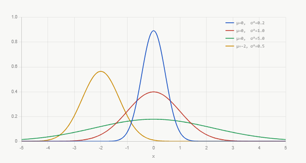
The probability density functions for several different means and standard deviations are shown above.
- $p(x)$ is the density of the probability at $x$, and not the probability. It can be greater than 1; it is the total area under the graph that must sum to 1.
-
To get the probability of $x$ falling within a range, take the integral under $p(x)$ for that specific range of $x$ values.
- The policy parametrization, defining the policy as the normal probability density over a real-valued scalar action $a$ with mean & standard deviation given by state-dependent, parametric function approximators, is as follows:
- The approximators need a representation form, so we split the policy’s parameter vector into 2 parts, $\boldsymbol{\theta} = [\boldsymbol{\theta}_{\mu}, \boldsymbol{\theta}_{\sigma}]^T$, one for mean approximation and the other for standard deviation approximation.
- The mean can be approximated as a linear function while the standard deviation can be approximated as the exponential of a linear function:
13.8 Summary
- Going from action-value methods to parametrized policy methods that take actions without consulting action-value estimates.
- More specifically, policy gradient methods update the policy parameter on each step in the direction of an estimate of the performance gradient w.r.t. the policy parameter.
- Advantages of parametrized policy methods over $\varepsilon$-greedy & action-value methods:
- They can learn specific probabilities for taking actions.
- They can learn appropriate levels of exploration & approach deterministic policies asymptotically.
- They can naturally handle continuous action spaces.
- Important theoretical advantage over action-value methods in the form of the policy gradient theorem.
- REINFORCE uses the policy gradient theorem with Monte Carlo returns.
- Addition of a state-value function as a baseline with REINFORCE reduces its variance without introducing bias and speeds up learning.
- If the state-value function is used to criticize/assess the policy’s action selections, then the value function is called a critic and the policy is called an actor. Overall this is referred to as the actor-critic method.
- The critic introduces bias into the actor’s gradient estimates, but is still often desirable for the same reason that bootstrapping TD methods are superior to Monte Carlo methods (significant variance reduction).
- Overall, policy-gradient methods provide a significantly different set of strengths & weaknesses than action-value methods.
Citation
If you found this blog post helpful, please consider citing it:
@article{obasi2026RLsuttonBartoCh13notes,
  title   = "Sutton & Barto, Ch. 13: Policy Gradient Methods (Personal Notes)",
  author  = "Obasi, Chizoba",
  journal = "chizkidd.github.io",
  year    = "2026",
  month   = "May",
  url     = "https://chizkidd.github.io/2026/05/07/rl-sutton-barto-notes-ch013/"
}