Sutton & Barto, Ch. 12: Eligibility Traces (Personal Notes)
- Eligibility traces are one of the basic mechanisms of RL that unify and generalize TD and Monte Carlo (MC) methods.
- TD methods augmented with eligibility traces produce a family of methods spanning a range from MC methods at one end ($\lambda = 1$) to one-step TD (TD(0)) methods at the other end ($\lambda = 0$).
- With eligibility traces, MC methods can be implemented online and on continuing problems.
- $n$-step methods also unify TD and MC methods but are not as elegant algorithmically as eligibility traces (ET).
- The eligibility traces algorithm entails:
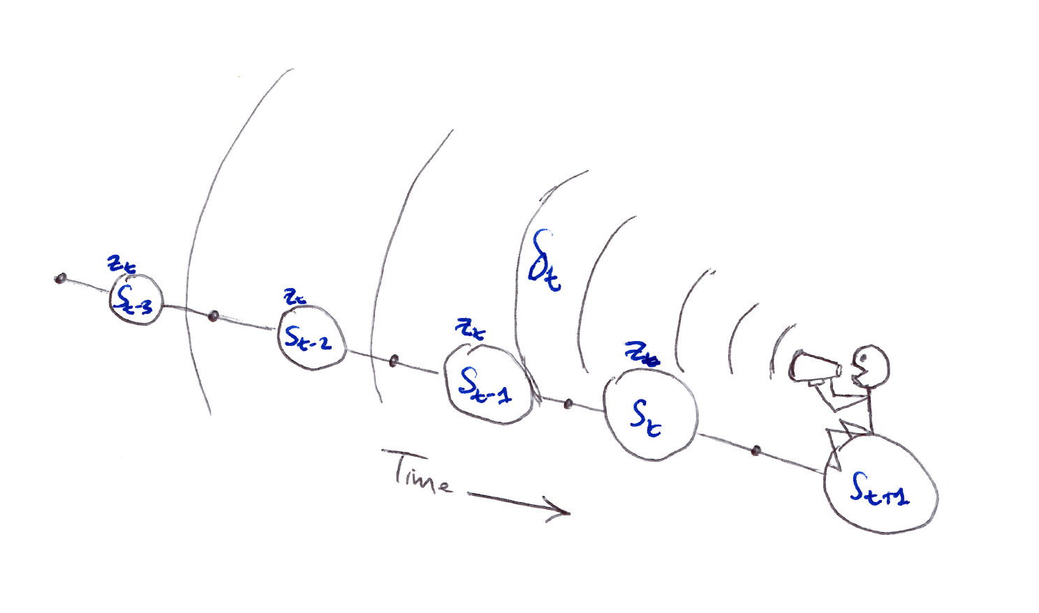
- First, we have a short-term memory vector, the eligibility trace $\mathbf{z}_t \in \mathbb{R}^d$, that parallels the long-term weight vector $\mathbf{w}_t \in \mathbb{R}^d$.
- Then when a component of $\mathbf{w}_t$ participates in producing an estimated value, the corresponding component of $\mathbf{z}_t$ is bumped up and then begins to fade away.
- Learning occurs in that component of $\mathbf{w}_t$ if a non-zero TD error occurs before the trace falls back to zero (fades away).
- The trace-decay parameter $\lambda \in [0,1)$ determines the rate at which the trace falls.
- Advantages of ET over $n$-step methods:
- Requires only a single trace vector $\mathbf{z}_t$ rather than storing the last $n$ feature vectors.
- Learning occurs continually and uniformly in time rather than being delayed and playing “catch up” at episode end. This leads to immediate behavior effect from learning rather than being delayed.
- ET is a backward view algorithm, unlike $n$-step methods that are forward view algorithms, which is less complex to implement.
- Forward view algorithms are based on looking forward from the updated state, and the updated state depends on all the future rewards.
- Backward view algorithms use the current TD error, looking backward to recently visited states, to achieve nearly the same updates as forward view.
- We start with ideas for state values and prediction, then extend them to action values and control, then do on-policy, then extend to off-policy learning. The field of focus is linear function approximation (covers tabular and state aggregation cases).
Table of Contents
- 12.1 The $\lambda$-return
- 12.2 TD($\lambda$)
- 12.3 $n$-step Truncated $\lambda$-return Methods
- 12.4 Redoing Updates: Online $\lambda$-return Algorithm
- 12.5 True Online TD($\lambda$)
- 12.6 Dutch Traces in Monte Carlo Learning
- 12.7 Sarsa($\lambda$)
- 12.8 Variable $\lambda$ and $\gamma$
- 12.9 Off-Policy Traces with Control Variates
- 12.10 Watkins’s Q($\lambda$) to Tree-Backup($\lambda$)
- 12.11 Stable Off-Policy Methods with Traces
- 12.12 Implementation Issues
- 12.13 Conclusions
Appendix
12.1 The $\lambda$-return
- Recall in Chapter 7 we defined an $n$-step return as the sum of the first $n$ rewards plus the estimated value of the state reached in $n$ steps, each appropriately discounted:
- A valid update can be done not just towards any $n$-step return, but also towards any average of $n$-step returns.
- E.g. average the 2-step and 4-step return: $\frac{1}{2} G_{t:t+2} + \frac{1}{2} G_{t:t+4}$
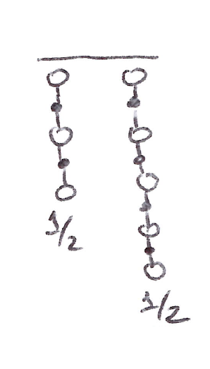
The compound update mixing half of a two-step return and half of a four-step return.
- Any set of $n$-step returns can be averaged, even an infinite set, as long as the weights on the component returns are positive and sum to $1$.
- What if instead of using one $n$-step return, we use a weighted average of all $n$-step returns? This leads to averaging which produces a substantial new range of algorithms.E.g.,
- Averaging one-step and infinite-step returns to interrelate TD and MC methods.
- Averaging experience-based updates with Dynamic Programming (DP) updates to obtain a single combination of experience-based and model-based methods.
- An update that averages simpler component updates is called a compound update or the $\lambda$-return.
- The TD($\lambda$) algorithm is one way of averaging $n$-step updates, each weighted proportionally by $\lambda^{n-1}$ (where $\lambda \in [0,1]$) and normalized by a factor of $(1-\lambda)$ to ensure that the weights sum to $1$.
If $\lambda = 0$, then the overall update reduces to its first component, the TD(0) update, whereas if $\lambda = 1$, then the overall update reduces to its last component, the MC update.
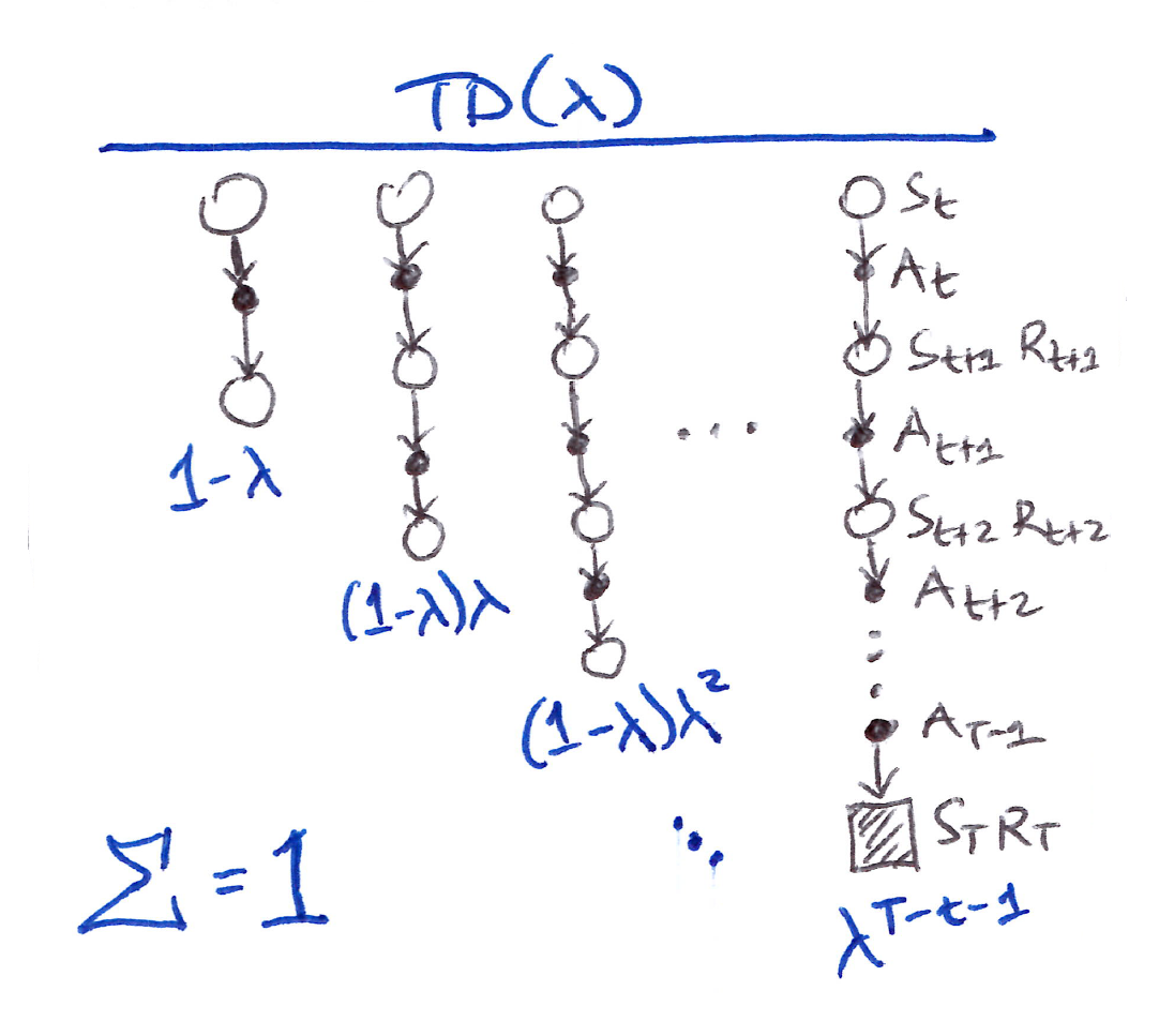
- Essentially, $\lambda$-return, $G_t^\lambda$, combines all $n$-step returns $G_{t:t+n}$ in a weighted average manner, $(1-\lambda)\lambda^{n-1}$, and is defined in its state-based form by:
TD($\lambda$) Weighting
- The TD($\lambda$) weighting function diagram illustrates the weighting on the sequence of $n$-step returns in the $\lambda$-return:
- $1$-step return gets the largest weight, $1-\lambda$
- $2$-step return gets the next (2nd) largest weight, $(1-\lambda)\lambda$
- $3$-step return gets the 3rd largest weight, $(1-\lambda)\lambda^2$
- $n$-step return gets the $n$-th largest (smallest) weight, $(1-\lambda)\lambda^{n-1}$
- The weight fades by $\lambda$ with each additional step.
- After a terminal state has been reached, all subsequent $n$-step returns are equal to the conventional return $G_t$.
- So essentially, we can decompose $G_t^\lambda$ based on the TD($\lambda$) weighting function diagram into the main sum and post-termination terms:
- So now we can see the impact of $\lambda$ more clearly:
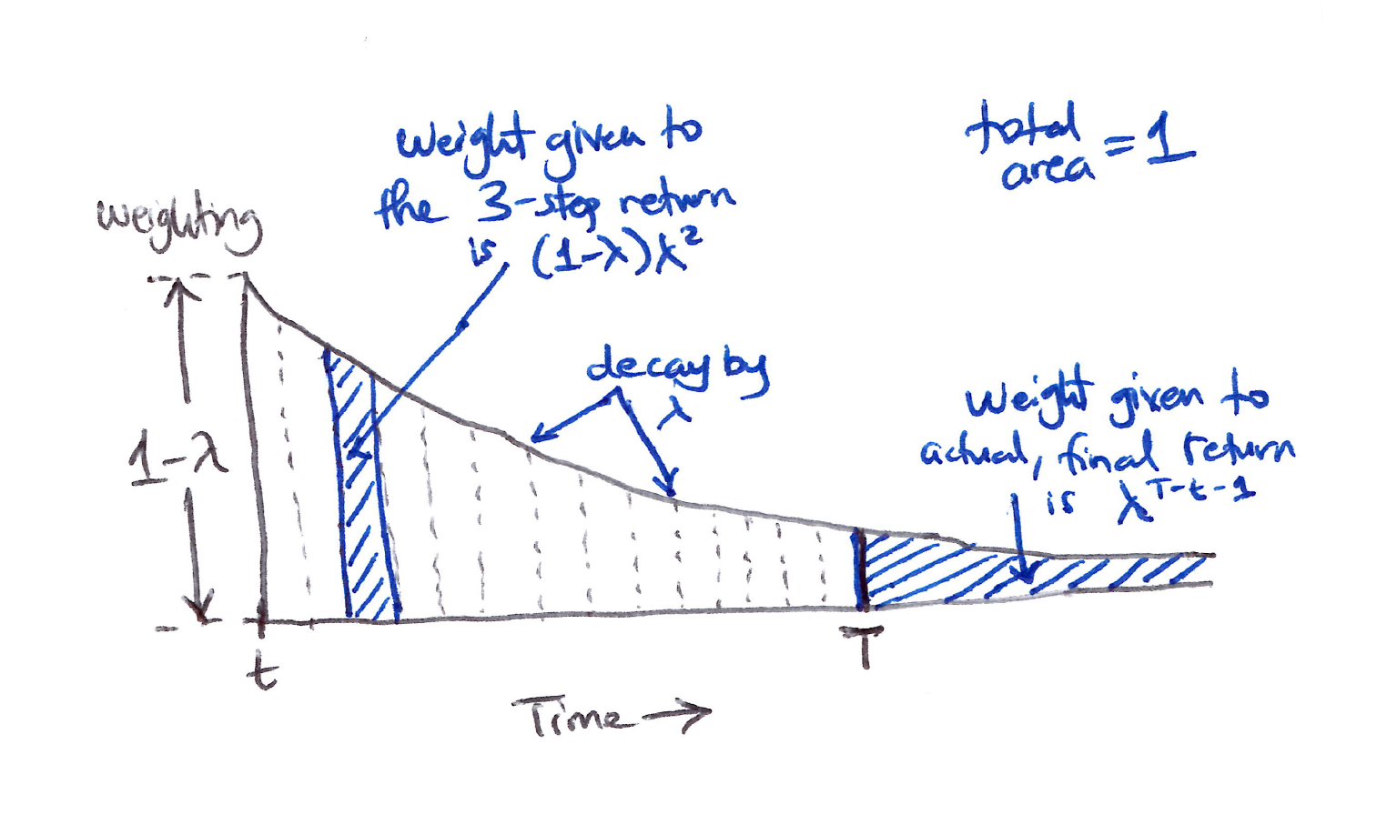
Weighting given in the $\lambda$-return to each of the $n$-step returns.
- Our first learning algorithm based on the $\lambda$-return is the off-line $\lambda$-return algorithm, which waits until the end of an episode to make updates. Its semi-gradient, $\lambda$-return, target update for $t = 0, 1, 2, \ldots, T-1$ is:
- The $\lambda$-return allows us to smoothly move between MC and TD(0) methods, comparable to $n$-step returning.
Forward View
- This approach is called the theoretical, forward view of a learning algorithm:
- Update value function towards the $\lambda$-return.
- Look forward in time to all the future rewards to compute $G_t^\lambda$.
- Like MC, can only be computed from complete return.
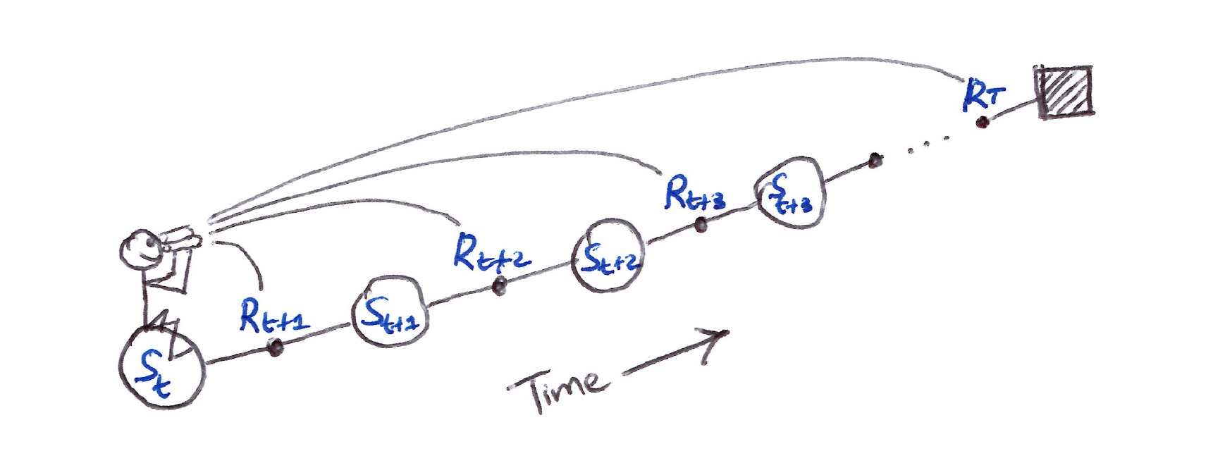
We decide how to update each state by looking forward to future rewards and states.
12.2 TD($\lambda$)
- TD($\lambda$) was the first algorithm that showed a formal relationship between a forward view and backward view using eligibility traces.
- TD($\lambda$) improves over the off-line $\lambda$-return algorithm in 3 ways:
- Updates the weight vector on every step of an episode and not just the end.
- Equal distributions in time of its computations rather than at an episode’s end.
- Can be applied to continuing problems and not just episodic problems.
- Let’s focus on the semi-gradient version of TD($\lambda$) with function approximation:
- The eligibility trace $\mathbf{z}_t$ has the same number of components as $\mathbf{w}_t$.
- $\mathbf{z}$ is initialized to $\mathbf{0}$, incremented on each time step by the value gradient, and then fades away by $\gamma\lambda$:
- The eligibility trace keeps track of which $\mathbf{w}_t$ components have contributed, positively or negatively, to recent state valuations.
- This is the recency heuristic used for credit assignment, where more credit is assigned to the most recent states. Recent is defined in terms of $\gamma\lambda$.
-
The TD error for state-value prediction is:
\[\delta_t \doteq R_{t+1} + \gamma \hat{v}(S_{t+1}, \mathbf{w}_t) - \hat{v}(S_t, \mathbf{w}_t)\]and the weight vector update in TD($\lambda$) is proportional to the scalar TD error and the vector eligibility trace:
Backward View
- Forward view provides theory but backward view provides mechanism (practical) where we update online, every step, from incomplete sequences.
- Keep an eligibility trace for every state $s$.
- Update value $V(s)$ for every state $s$ in proportion to TD-error $\delta_t$ and eligibility trace $\mathbf{z}_t$:
In the backward or mechanistic view of TD($\lambda$), each update depends on the current TD error combined with the current eligibility traces of past events.
- Let’s look at the effect of $\lambda$ to understand the backward view of TD($\lambda$):
-
In summary, $\lambda = 1$ yields TD(1).
- TD(1) implements MC algorithms in a more general way and for a wider range of applicability:
- Not limited to episodic tasks, can be applied to discounted continuing tasks.
- Can be performed incrementally and online.
- Learns immediately and alters behavior during an episode if something good or bad happens, for control methods.
- Linear TD($\lambda$) converges in the on-policy case if the step-size parameter $\alpha$ is reduced over time according to stochastic approximation theory conditions.
- The convergence of linear TD($\lambda$) is not to the minimum-error weight vector but to a nearby weight vector that depends on $\lambda$.
- The bound on solution quality generalized for any $\lambda$, for the continuing, discounted case is:
- That is, the asymptotic error is no more than $\dfrac{1-\gamma\lambda}{1-\gamma}$ times the smallest possible error for TD($\lambda$):
- However, $\lambda = 1$ is often the poorest choice.
12.3 $n$-step Truncated $\lambda$-return Methods
- The off-line $\lambda$-return is of limited use because the $\lambda$-return is not known until the episode ends.
- The off-line $\lambda$-return approximation is to truncate the sequence after a fixed number of steps.
- Hence, a natural approximation is to truncate the sequence where $\lambda$-return cannot be calculated for an arbitrarily large $n$. This handles the continuing case.
- The truncated $\lambda$-return for time $t$, given data only up to some later horizon $h$, is:
- Here the residual weighting is given to the longest available $n$-step return $G_{t:h}$.
- The truncated $\lambda$-return gives rise to a family of $n$-step $\lambda$-return algorithms, known in the state-value case as Truncated TD($\lambda$) or TTD($\lambda$).
- TTD($\lambda$) is defined for $0 \leq t < T$ by:
- Efficient implementation of TTD($\lambda$) relies on the $k$-step $\lambda$-return:
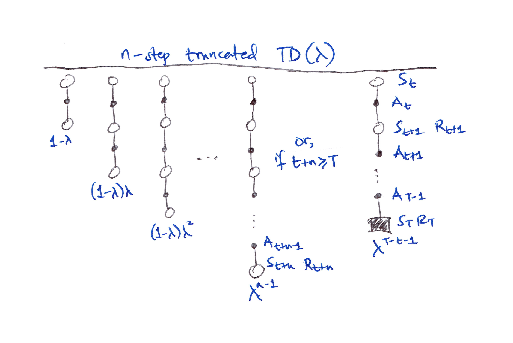
The truncated $\lambda$-return gives rise to a family of $n$-step $\lambda$-return algorithms called TTD($\lambda$).
12.4 Redoing Updates: Online $\lambda$-return Algorithm
- How do we choose the truncation parameter $n$ in TTD($\lambda$)?
- It involves a tradeoff:
- $n$ should be large so that TTD($\lambda$) closely approximates off-line $\lambda$-return, but
- $n$ should also be small so that the updates can be made sooner and can influence behavior sooner.
- In principle, we can achieve both cases via the online $\lambda$-return algorithm, but at the cost of computational complexity.
- Essentially at each time step, we go back and redo all the updates since the beginning of the episode as we gather new increment of data:
- The new updates are better than the old ones because now they account for the time step’s new data.
- Basically this conceptual algorithm involves multiple passes over the episode, one at each horizon, each generating a different sequence of weight vectors.
- Let’s distinguish between the weight vectors computed at the different horizons by seeing the first 3 sequences:
- The general form of the online $\lambda$-return update for $0 \leq t < h \leq T$ is:
12.5 True Online TD($\lambda$)
- The original ideal online $\lambda$-return algorithm shown in Section 12.4 is very complex so we use online TD($\lambda$) to approximate it.
- We’ll use eligibility trace to invert the forward view, online $\lambda$-return to an efficient backward view algorithm. This is called the True Online TD($\lambda$).
- It uses a simple strategy trick with the weight matrix, where we only need to keep the last weight vector from all the updates at the last time step (the diagonals of online $\lambda$-return weight matrix).
- For the linear case in which $\hat{v}(s, \mathbf{w}) = \mathbf{w}^T \mathbf{x}(s)$, the true online TD($\lambda$) algorithm is:
- The per-step computational complexity of true online TD($\lambda$) is the same as TD($\lambda$), $O(d)$.
- $\mathbf{z}_t$ used in true online TD($\lambda$) is called a dutch trace, unlike that of TD($\lambda$) which is called an accumulating trace.
- Earlier work used a 3rd kind of trace called the replacing trace, defined only for the tabular case or for binary feature vectors (tile coding). It is defined:
- Nowadays, dutch traces usually perform better than replacing traces and have a clearer theoretical basis.
- Accumulating traces remain of interest for nonlinear function approximations where dutch traces are unavailable.
12.6 Dutch Traces in Monte Carlo Learning
- Eligibility traces have nothing to do with TD learning despite their close historical association.
- Eligibility traces arise even in Monte Carlo learning.
- Using dutch traces, we can invert the forward view MC algorithm to an equivalent, yet computationally cheaper backward view algorithm.
-
This is the only equivalence of forward and backward view that is explicitly demonstrated in this book.
- The linear, gradient MC prediction algorithm makes the following sequence of updates, one for each time step of the episode:
- For simplicity, assume that the return $G$ is a single reward at the end of the episode (hence no subscript by time) and that there is no discounting.
- This is known as the Least Mean Square (LMS) rule.
-
We introduce an additional vector memory, the eligibility trace, that keeps in it a summary of all the feature vectors seen so far. The overall update will be the same as the MC updates’ sequence shown above and is:
\[\begin{align*} \mathbf{w}_T &= \mathbf{w}_{T-1} + \alpha \!\left(G - \mathbf{w}_{T-1}^T \mathbf{x}_{T-1}\right) \mathbf{x}_{T-1} \\ &= \mathbf{w}_{T-1} + \alpha \mathbf{x}_{T-1}\!\left(-\mathbf{x}_{T-1}^T \mathbf{w}_{T-1}\right) + \alpha G \mathbf{x}_{T-1} \\ &= \!\left(\mathbf{I} - \alpha \mathbf{x}_{T-1} \mathbf{x}_{T-1}^T\right) \mathbf{w}_{T-1} + \alpha G \mathbf{x}_{T-1} \\ &= \mathbf{F}_{T-1}\, \mathbf{w}_{T-1} + \alpha G \mathbf{x}_{T-1} \end{align*}\] \[\begin{aligned} \text{where} \\ \mathbf{F}_t &\doteq \mathbf{I} - \alpha \mathbf{x}_t \mathbf{x}_t^T \equiv \text{a forgetting or fading matrix} \end{aligned}\] \[\therefore\quad \mathbf{w}_{T-1} = \mathbf{F}_{T-2}\, \mathbf{w}_{T-2} + \alpha G \mathbf{x}_{T-2}\]Now recursing:
\[\begin{align*} \mathbf{w}_T &= \mathbf{F}_{T-1}\, \mathbf{w}_{T-1} + \alpha G \mathbf{x}_{T-1} \\ &= \mathbf{F}_{T-1}\!\left(\mathbf{F}_{T-2}\, \mathbf{w}_{T-2} + \alpha G \mathbf{x}_{T-2}\right) + \alpha G \mathbf{x}_{T-1} \\ &= \mathbf{F}_{T-1} \mathbf{F}_{T-2}\, \mathbf{w}_{T-2} + \alpha G\!\left(\mathbf{F}_{T-1} \mathbf{x}_{T-2} + \mathbf{x}_{T-1}\right) \\ &= \mathbf{F}_{T-1} \mathbf{F}_{T-2}\!\left(\mathbf{F}_{T-3}\, \mathbf{w}_{T-3} + \alpha G\, \mathbf{x}_{T-3}\right) + \alpha G\!\left(\mathbf{F}_{T-1}\, \mathbf{x}_{T-2} + \mathbf{x}_{T-1}\right) \\ &= \mathbf{F}_{T-1} \mathbf{F}_{T-2} \mathbf{F}_{T-3}\, \mathbf{w}_{T-3} + \alpha G\!\left(\mathbf{F}_{T-1} \mathbf{F}_{T-2}\, \mathbf{x}_{T-3} + \mathbf{F}_{T-1}\, \mathbf{x}_{T-2} + \mathbf{x}_{T-1}\right) \\ &\quad \vdots \\ &= \underbrace{\mathbf{F}_{T-1} \mathbf{F}_{T-2} \cdots \mathbf{F}_0\, \mathbf{w}_0}_{\mathbf{a}_{T-1}} + \alpha G \underbrace{\sum\nolimits_{k=0}^{T-1} \mathbf{F}_{T-1} \mathbf{F}_{T-2} \cdots \mathbf{F}_{k+1}\, \mathbf{x}_k}_{\mathbf{z}_{T-1}} \\ &= \mathbf{a}_{T-1} + \alpha G\, \mathbf{z}_{T-1} \end{align*}\] \[\begin{aligned} \text{where} \\ \mathbf{a}_{T-1}\ \&\ \mathbf{z}_{T-1} &\equiv \text{values at time } T-1 \text{ of 2 auxiliary memory vectors that can be updated} \\ &\phantom{{}\equiv{}} \text{incrementally w/o knowledge of } G \text{ and with } O(d) \text{ complexity per time step} \\ \mathbf{z}_t &\equiv \text{dutch-style eligibility trace, initialized to } \mathbf{z}_0 = \mathbf{x}_0 \end{aligned}\] -
The $\mathbf{z}_t$ vector is in fact a dutch-style eligibility trace, initialized to $\mathbf{z}_0 = \mathbf{x}_0$, that can be updated according to:
\[\begin{align*} \mathbf{z}_t &= \sum\nolimits_{k=0}^{t} \mathbf{F}_t \mathbf{F}_{t-1} \cdots \mathbf{F}_{k+1}\, \mathbf{x}_k, \quad 1 \leq t < T \\ &= \sum\nolimits_{k=0}^{t-1} \mathbf{F}_t \mathbf{F}_{t-1} \cdots \mathbf{F}_{k+1}\, \mathbf{x}_k + \mathbf{x}_t \\ &= \mathbf{F}_t \sum\nolimits_{k=0}^{t-1} \mathbf{F}_{t-1} \mathbf{F}_{t-2} \cdots \mathbf{F}_{k+1}\, \mathbf{x}_k + \mathbf{x}_t \\ &= \mathbf{F}_t\, \mathbf{z}_{t-1} + \mathbf{x}_t \\ &= \!\left(\mathbf{I} - \alpha \mathbf{x}_t \mathbf{x}_t^T\right) \mathbf{z}_{t-1} + \mathbf{x}_t \\ &= \mathbf{z}_{t-1} - \alpha\!\left(\mathbf{z}_{t-1}^T \mathbf{x}_t\right) \mathbf{x}_t + \mathbf{x}_t \\ &\boxed{= \mathbf{z}_{t-1} + \!\left(1 - \alpha\, \mathbf{z}_{t-1}^T \mathbf{x}_t\right) \mathbf{x}_t} \end{align*}\]which is the dutch trace for $\gamma\lambda = 1$.
-
The $\mathbf{a}_t$ auxiliary vector is initialized to $\mathbf{a}_0 = \mathbf{w}_0$ and then updated according to:
\[\begin{align*} \mathbf{a}_t &= \mathbf{F}_t \mathbf{F}_{t-1} \cdots \mathbf{F}_0\, \mathbf{w}_0, \quad 1 \leq t < T \\ &= \mathbf{F}_t\, \mathbf{a}_{t-1} \\ &= \mathbf{a}_{t-1} - \alpha \mathbf{x}_t \mathbf{x}_t^T \mathbf{a}_{t-1} \\ &\boxed{= \mathbf{a}_{t-1}\!\left(\mathbf{I} - \alpha \mathbf{x}_t \mathbf{x}_t^T\right)} \end{align*}\]
Takeaways
- The auxiliary vectors, $\mathbf{a}_t$ and $\mathbf{z}_t$, are updated on each time step $t < T$ and then, at time $T$ when $G$ is observed, they are used to compute:
- The time and memory complexity per step is $O(d)$.
- This is surprising and intriguing since ET is working in a non-TD setting (ET arise where long-term predictions are needed to be learned efficiently).
12.7 Sarsa($\lambda$)
- Now let’s extend eligibility traces to action-value methods.
-
First, let’s recall the action-value form of the $n$-step return:
\[G_{t:t+n} \doteq R_{t+1} + \ldots + \gamma^{n-1} R_{t+n} + \gamma^n \hat{q}(S_{t+n}, A_{t+n}, \mathbf{w}_{t+n-1}), \quad t+n < T\] \[\text{with} \quad G_{t:t+n} = G_t \quad \text{ if } t+n \geq T.\] - With this, for $t = 0, \ldots, T-1,$ let’s form the action-value form of the off-line $\lambda$-return algorithm which uses $\hat{q}$ rather than $\hat{v}$:
- For the forward view shown in the figure below, which is similar to TD($\lambda$), the updates are:
- 1st update: one full-step lookahead
- 2nd update: two-step lookahead
- Final update: complete return.
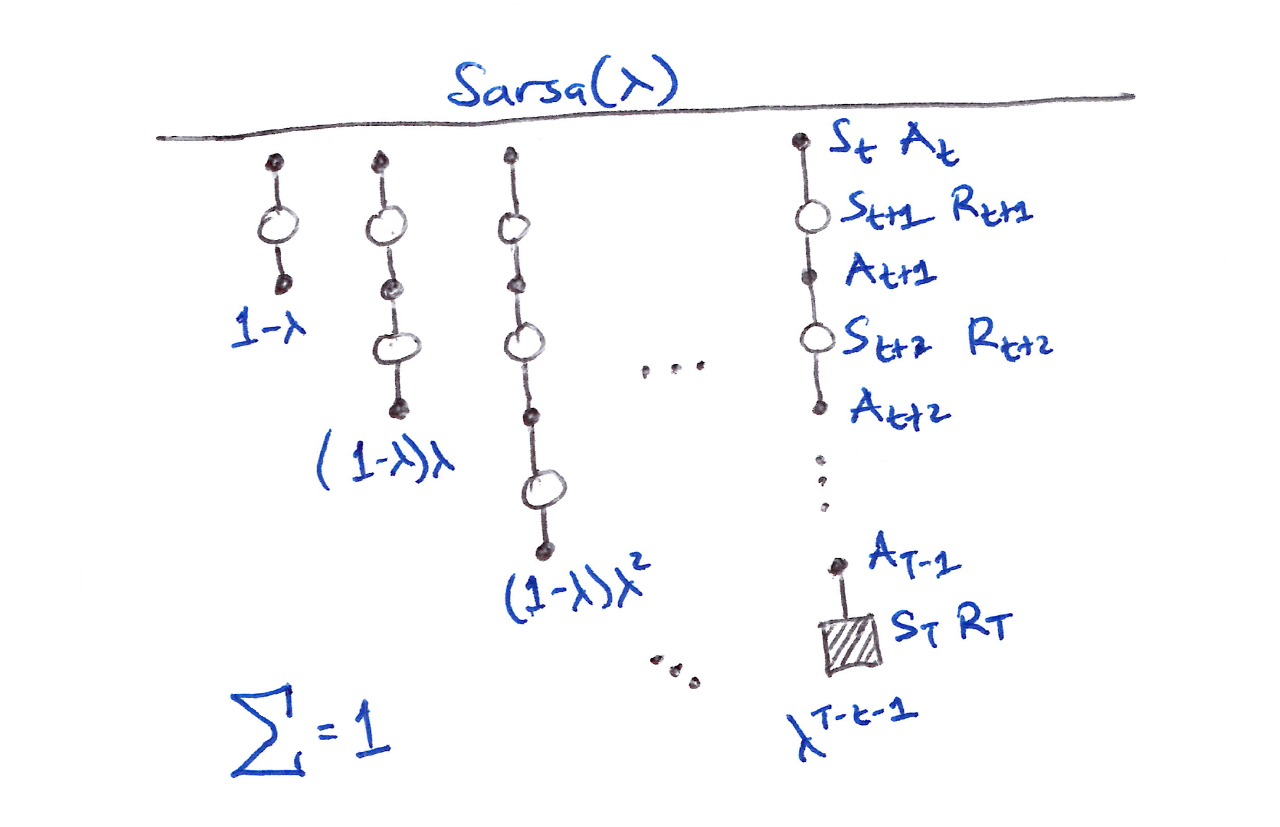
The first update looks ahead one full step, to the next state–action pair, the second looks ahead two steps, to the second state–action pair, and so on. A final update is based on the complete return.
- The weighting of each $n$-step update in the $\lambda$-return is same as in TD($\lambda$) and $\lambda$-return.
- The forward view TD for action values, Sarsa($\lambda$), has the same update rule as TD($\lambda$):
- The action-value form of the TD error is used:
- The action-value form of the eligibility trace:
- There exists an action-value version of our ideal TD method, the online $\lambda$-return algorithm and its efficient implementation as true online TD($\lambda$):
- Section 12.4: Everything there holds here except for using the action-value form of the $n$-step return, $G_{t:t+n}$.
- Sections 12.5 & 12.6: Everything holds here except for using state-action feature vectors $\mathbf{x}_t = \mathbf{x}(S_t, A_t)$ instead of state feature vectors $\mathbf{x}_t = \mathbf{x}(S_t)$.
- The resulting efficient backward algorithm obtained from using the eligibility trace to invert the action-value form of the forward view, online $\lambda$-return is called the True Online Sarsa($\lambda$).
- There is also a truncated version of Sarsa($\lambda$), called Forward Sarsa($\lambda$), which appears to be a model-free, control method for use in conjunction with multi-layer ANNs.
12.8 Variable $\lambda$ and $\gamma$
- To get the most general forms of the final TD algorithms, it is vital to generalize the degree of bootstrapping and discounting beyond constant parameters to functions dependent on the state and action:
- $\lambda_t$ is the termination function and is significant because it changes the return $G_t$, which is now more generally defined as:
- This general return $G_t$ definition enables episodic settings to become a single stream of experience, without special terminal state, start distributions or termination times
- A terminal state just becomes a state with $\gamma(s) = 0$ that transitions to the start distribution.
- Generalization to variable bootstrapping yields a new state-based $\lambda$-return:
- Action-based $\lambda$-return is either the Sarsa form:
- or the Expected Sarsa form:
Superscripts notation for $i$ in $G_t^{\lambda i}$
\[\begin{aligned} \text{"s"} &: \text{bootstraps from state values} \\ \text{"a"} &: \text{bootstraps from action values} \end{aligned}\]12.9 Off-Policy Traces with Control Variates
- To generalize to off-policy, we need to incorporate importance sampling using eligibility traces.
- Let’s focus on the bootstrapping generalization of per-decision importance sampling with control variates (Section 7.4).
- The new state-based $\lambda$-return in Section 12.8 generalizes, after the off-policy, control variate, $n$-step return (ending at horizon $h$) model to:
- The final $\lambda$-return can be approximated in terms of sums of the state-based TD error $\delta_t^s$, with the approximation becoming exact if the approximate value function does not change:
- The forward view update of the approximate $\lambda$-return is:
- We’re interested in the equivalence (approximately) between the forward-view update summed over time and a backward-view update summed over time. The equivalence is approximate because we ignore changes in the value function.
- The sum of the forward-view update over time is:
- If the entire expression from the 2nd sum on could be written and updated incrementally as an eligibility trace, then the sum of the forward-view update over time would be in the form of the sum of a backward-view TD update.
- That is, if this expression was the trace at time $k$, then we could update it from its value at time $k-1$ by:
- If we change the index from $k$ to $t$ of the $\mathbf{z}_k$ equation above, we get the general accumulating trace update for state values:
- This eligibility trace combined with the usual semi-gradient TD($\lambda$) parameter-update rule (Section 12.2) forms a general TD($\lambda$) algorithm that can be applied to either on-policy or off-policy data:
- In on-policy, the algorithm is exactly TD($\lambda$) because $\rho_t = 1$ always and the ET above becomes the usual accumulating trace for variable $\lambda$ and $\gamma$:
- In off-policy, the algorithm stays as it is, although not guaranteed to be stable as a semi-gradient method.
- For off-policy, we’ll consider extensions that guarantee stability in the next few sections.
- Let’s derive the off-policy ET for action-value methods and corresponding general Sarsa($\lambda$) algorithms.
- Starting with either recursive general action-based $\lambda$-return of Sarsa or Expected Sarsa, $G_t^{\lambda a}$, in Section 12.8 (Expected Sarsa works out to be simpler), we can extend the Expected Sarsa $G_t^{\lambda a}$ to the off-policy case after the off-policy model of action-based, off-policy, control variate, $n$-step return:
- The $\lambda$-return, approximately as the sum of TD errors, is:
- Using steps analogous to those for the state case earlier in this section, write a forward-view update based on action-based $\lambda$-return $G_t^{\lambda a}$ above, then transform the sum of the updates using the summation rule and finally derive the eligibility trace for action values:
- This ET combined with the action-based, expected TD error $\delta_t^a$ and the usual semi-gradient TD($\lambda$) parameter-update rule (Section 12.2) forms an elegant, efficient Expected Sarsa($\lambda$) algorithm that can be applied to either on-policy or off-policy data:
- On-policy case: The algorithm becomes the Sarsa($\lambda$) algorithm given constant $\lambda$ and $\gamma$, and the usual state-action TD error:
- At $\lambda = 1$, these algorithms become closely related to corresponding Monte Carlo algorithms.
- No episode-by-episode equivalence of updates exist, only of their expectations, even under the most favorable conditions.
- Methods have been proposed recently [Sutton, Mahmood, Precup & van Hasselt, 2014] that do achieve an exact equivalence.
- These methods require an additional vector of “provisional weights” that keep track of executed updates but may need to be retracted/emphasized depending on future actions taken.
- The state and state-action versions of these methods are called PTD($\lambda$) and PQ($\lambda$) respectively, where the ‘P’ stands for Provisional.
-
If $\lambda < 1$, then all these off-policy algorithms involve bootstrapping and the deadly triad applies, meaning that they can be guaranteed stable only for the tabular case, state aggregation and other limited forms of function approximation.
- Recall the challenge of off-policy learning has 2 parts. Off-policy eligibility traces deal effectively with the 1st part, correcting for the expected value of the targets, but not with the 2nd part that has to do with distribution of updates (matching off-policy to on-policy).
- Algorithmic strategies for handling the 2nd part of the off-policy learning challenge with eligibility traces are summarized in Section 12.11.
12.10 Watkins’s Q($\lambda$) to Tree-Backup($\lambda$)
Watkins’s Q($\lambda$)
- Watkins’s Q($\lambda$) is the original method for extending Q-learning to eligibility traces.
- It involves decaying the ET in the usual way as long as a greedy action was taken, then cuts the traces to 0 after the 1st non-greedy action.
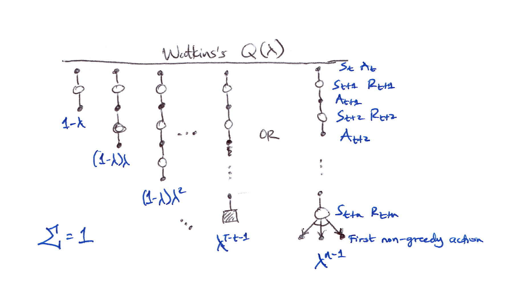
The series of component updates ends either with the end of the episode or with the first nongreedy action, whichever comes first.
Tree-Backup($\lambda$)
- Let’s look at the eligibility trace version of Tree Backup, which is called Tree-Backup($\lambda$) or TB($\lambda$).
- TB($\lambda$) is the true successor to Q-learning because it has no importance sampling.
- TB($\lambda$) concept is straightforward:
-
The tree-backup updates of each length (Section 7.5) are weighted dependent on the bootstrapping parameter $\lambda$.
-
Using the recursive form of the action-based $\lambda$-return for Expected Sarsa and then expanding the bootstrapping target case after the model of tree-backup $n$-step return (Section 7.5):
\[\boxed{\begin{align*} G_t^{\lambda a} &\doteq R_{t+1} + \gamma_{t+1}\!\left(\!\left[1 - \lambda_{t+1}\right] \bar{V}_t(S_{t+1}) + \lambda_{t+1}\!\left[\sum_{a \neq A_{t+1}} \pi(a \vert S_{t+1})\, \hat{q}(S_{t+1}, a, \mathbf{w}_t) + \pi(A_{t+1} \vert S_{t+1}) G_{t+1}^{\lambda a}\right]\right) \\ &= R_{t+1} + \gamma_{t+1}\!\left(\bar{V}_t(S_{t+1}) + \lambda_{t+1} \pi(A_{t+1} \vert S_{t+1}) \!\left[G_{t+1}^{\lambda a} - \hat{q}(S_{t+1}, A_{t+1}, \mathbf{w}_t)\right]\right) \end{align*}}\]
-
-
$G_t^{\lambda a}$ can be approximated (ignoring changes in approx. value function) as a sum of TD errors:
\[\begin{align*} G_t^{\lambda a} &\approx \hat{q}(S_t, A_t, \mathbf{w}_t) + \sum_{k=t}^{\infty} \delta_k^a \prod_{i=t+1}^{k} \gamma_i \lambda_i \pi(A_i \vert S_i) \\ \delta_t^a &= R_{t+1} + \gamma_{t+1} \bar{V}_t(S_{t+1}) - \hat{q}(S_t, A_t, \mathbf{w}_t) \end{align*}\] -
As always, using same steps as in the previous section, we get a special eligibility trace update involving the target-policy probabilities of the selected actions:
\[\boxed{\mathbf{z}_t \doteq \gamma_t \lambda_t \pi(A_t \vert S_t)\, \mathbf{z}_{t-1} + \nabla \hat{q}(S_t, A_t, \mathbf{w}_t)}\]
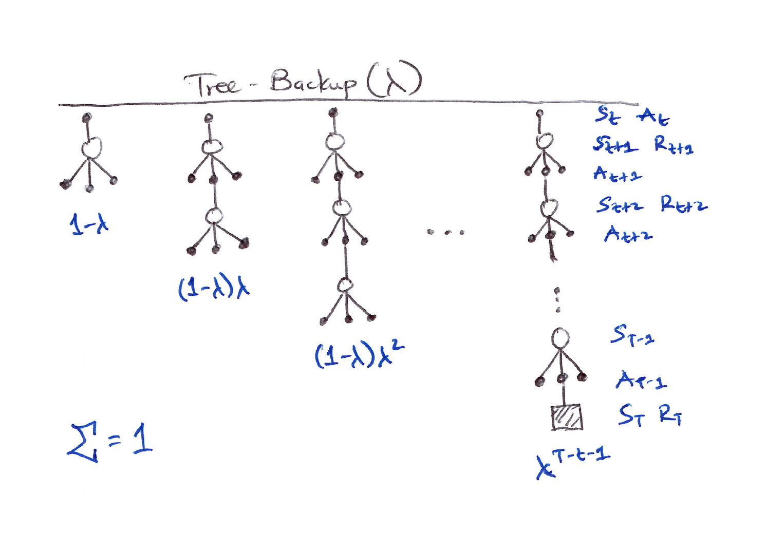
The tree-backup updates of each length are weighted in the usual way dependent on the bootstrapping parameter $\lambda$
- The ET above combined with the usual semi-gradient TD($\lambda$) parameter-update rule defines the TB($\lambda$) algorithm.
- Like all semi-gradient algorithms, TB($\lambda$) is not guaranteed to be stable when used with off-policy data and a powerful function approximator (the deadly triad).
12.11 Stable Off-Policy Methods with Traces
- Let’s look at 4 of the most important methods that achieve stable off-policy methods/training using eligibility traces.
- All 4 are based on either the Gradient-TD or Emphatic TD and linear function approximation.
GTD($\lambda$)
-
Analogous to TDC, and aims to learn a parameter $\mathbf{w}_{t}$ such that $\hat{v}(s, \mathbf{w}) \doteq \mathbf{w}_{t}^T \mathbf{x}(s) \approx v_{\pi}(s)$ even from data that is due to following another policy $b$. Its update is:
\[\begin{aligned} \mathbf{w}_{t+1} &\doteq \mathbf{w}_t + \alpha\, \delta_t^s\, \mathbf{z}_t - \alpha \gamma_{t+1}(1 - \lambda_{t+1})\!\left(\mathbf{z}_t^T \mathbf{v}_t\right) \mathbf{x}_{t+1} \\ \mathbf{v}_{t+1} &\doteq \mathbf{v}_t + \beta\, \delta_t^s\, \mathbf{z}_t - \beta\!\left(\mathbf{v}_t^T \mathbf{x}_t\right) \mathbf{x}_t \end{aligned}\] \[\begin{aligned} \text{where} \\ \mathbf{v} &\in \mathbb{R}^d \equiv \text{a vector of the same dimension as } \mathbf{w}, \text{ initialized to } \mathbf{v}_0 = \mathbf{0} \\ \beta &> 0 \equiv \text{a 2nd step-size parameter} \end{aligned}\]
GQ($\lambda$)
- Gradient-TD algorithm for action values with eligibility traces.
- GQ($\lambda$) aims to learn $\mathbf{w}_{t}$ such that $\hat{q}(s, a, \mathbf{w}_{t}) \doteq \mathbf{w}_{t}^T \mathbf{x}(s,a) \approx q_{\pi}(s,a)$ from off-policy data.
- If the target policy is $\varepsilon$-greedy, or otherwise biased towards the greedy policy for $\hat{q}$, then GQ($\lambda$) can be used as a control algorithm.
-
GQ($\lambda$) update is:
\[\begin{aligned} \mathbf{w}_{t+1} &\doteq \mathbf{w}_t + \alpha\, \delta_t^a\, \mathbf{z}_t - \alpha \gamma_{t+1}(1 - \lambda_{t+1})\!\left(\mathbf{z}_t^T \mathbf{v}_t\right) \bar{\mathbf{x}}_{t+1} \\ \bar{\mathbf{x}}_t &\doteq \sum_a \pi(a \vert S_t)\, \mathbf{x}(S_t, a) \\ \delta_t^a &\doteq R_{t+1} + \gamma_{t+1}\, \mathbf{w}_t^T \bar{\mathbf{x}}_{t+1} - \mathbf{w}_t^T \mathbf{x}_t \\ \mathbf{z}_t &\doteq \gamma_t \lambda_t \rho_t\, \mathbf{z}_{t-1} + \nabla \hat{q}(S_t, A_t, \mathbf{w}_t) \end{aligned}\] \[\begin{aligned} \text{where} \\ \bar{\mathbf{x}}_t &\equiv \text{average feature vector for } S_t \text{ under the target policy} \\ \delta_t^a &\equiv \text{expectation form of the TD error} \end{aligned}\]
HTD($\lambda$)
- Hybrid TD($\lambda$) state-value algorithm combines aspects of GTD($\lambda$) and TD($\lambda$).
-
HTD($\lambda$) is a strict generalization of TD($\lambda$) to the off-policy setting, meaning it reduces exactly to TD($\lambda$) when the behavior and target policies coincide; a property GTD($\lambda$) does not share:
\[b(A_t \vert S_t) = \pi(A_t \vert S_t), \quad \rho_t = 1 \implies \text{HTD}(\lambda) = \text{TD}(\lambda)\] -
HTD($\lambda$) is defined by:
\[\begin{aligned} \mathbf{w}_{t+1} &\doteq \mathbf{w}_t + \alpha\, \delta_t^s\, \mathbf{z}_t + \alpha\!\left[\!\left(\mathbf{z}_t - \mathbf{z}_t^b\right)^T \mathbf{v}_t\right]\!\left(\mathbf{x}_t - \gamma_{t+1} \mathbf{x}_{t+1}\right) \\ \mathbf{v}_{t+1} &\doteq \mathbf{v}_t + \beta\, \delta_t^s\, \mathbf{z}_t - \beta\!\left(\mathbf{z}_t^T \mathbf{v}_t\right)\!\left(\mathbf{x}_t - \gamma_{t+1} \mathbf{x}_{t+1}\right), \quad & \mathbf{v}_0 \doteq \mathbf{0} \\ \mathbf{z}_t &\doteq \rho_t \!\left(\gamma_t \lambda_t\, \mathbf{z}_{t-1} + \mathbf{x}_t\right), \quad & \mathbf{z}_{-1} \doteq \mathbf{0} \\ \mathbf{z}_t^b &\doteq \gamma_t \lambda_t\, \mathbf{z}_{t-1}^b + \mathbf{x}_t, \quad & \mathbf{z}_{-1}^b \doteq \mathbf{0} \end{aligned}\] - We get
- a 2nd set of weights, $\mathbf{v}_t$.
- a 2nd set of eligibility traces, $\mathbf{z}_t^b$, conventional accumulating traces for the behavior policy.
Emphatic TD($\lambda$)
- Extension of one-step Emphatic TD (Sections 9.11 & 11.8) to eligibility traces.
- The resulting algorithm:
- (+) retains strong off-policy convergence guarantees
- (+) enables any degree of bootstrapping
- (-) has high variance
- (-) potentially slow convergence.
-
Emphatic TD($\lambda$) is defined by:
\[\begin{aligned} \mathbf{w}_{t+1} &\doteq \mathbf{w}_t + \alpha\, \delta_t\, \mathbf{z}_t \\ \delta_t &\doteq R_{t+1} + \gamma_{t+1}\, \mathbf{w}_t^T \mathbf{x}_{t+1} - \mathbf{w}_t^T \mathbf{x}_t \\ \mathbf{z}_t &\doteq \rho_t \!\left(\gamma_t \lambda_t\, \mathbf{z}_{t-1} + M_t \mathbf{x}_t\right), \quad & \mathbf{z}_{-1} \doteq \mathbf{0} \\ M_t &\doteq \lambda_t \mathcal{I}_t + (1 - \lambda_t) F_t \\ F_t &\doteq \rho_{t-1} \gamma_t F_{t-1} + \mathcal{I}_t, \quad & F_0 \doteq \mathcal{i}(S_0) \end{aligned}\] \[\begin{aligned} \text{where} \\ M_t &\geq 0 \equiv \text{emphasis} \\ F_t &\geq 0 \equiv \text{followon trace} \\ \mathcal{I}_t &\geq 0 \equiv \text{interest} \end{aligned}\] - In the on-policy case ($\rho_t = 1$ for all $t$), Emphatic TD($\lambda$) is similar to conventional TD($\lambda$), but still significantly different:
- Emphatic TD($\lambda$) is guaranteed to converge for all state-dependent $\lambda$ functions; TD($\lambda$) is not (TD($\lambda$) is guaranteed only for constant $\lambda$).
- See Yu’s counterexample [Ghassian, Rafiee & Sutton, 2016].
12.12 Implementation Issues
- Naive implementation seems expensive: Updating eligibility traces for every state at every time step appears computationally costly on serial computers.
- Practical optimization: Most ET are nearly 0; only recently visited states have significant traces, so implementations can track and update only these few states.
- Computational cost: With this optimization, tabular methods with traces are only a few times more expensive than one-step methods.
- Function approximation reduces overhead: When using neural networks, ET typically only double memory and computation per step (much less overhead than in tabular case).
- Tabular is the worst case: The tabular setting represents the highest computational complexity for ET relative to simpler methods.
12.13 Conclusions
- Eligibility traces provide an efficient, incremental way to interpolate between TD and MC methods.
- ET offer advantages over $n$-step methods in terms of generality and computational trade-offs.
- Empirically, an intermediate mix works best: ET should move towards MC but not all the way since pure MC performance degrades sharply.
- ET are the first defense against long-delayed rewards and non-Markov tasks, used with TD methods to make them behave more like MC methods without full bootstrapping.
- Use traces when data is scarce and online learning is required, as they provide faster learning per sample despite higher computational cost per step.
- Avoid traces in offline settings with cheap abundant data (maximum data processing speed matters more than learning efficiency per sample).
- True online methods achieve ideal $\lambda$-return performance while maintaining $O(d)$ computational efficiency.
- Forward-to-backward view derivations provide computationally efficient, mechanistic, practical implementations of theory.
Citation
If you found this blog post helpful, please consider citing it:
@article{obasi2026RLsuttonBartoCh12notes,
  title   = "Sutton & Barto, Ch. 12: Eligibility Traces (Personal Notes)",
  author  = "Obasi, Chizoba",
  journal = "chizkidd.github.io",
  year    = "2026",
  month   = "Mar",
  url     = "https://chizkidd.github.io/2026/03/13/rl-sutton-barto-notes-ch012/"
}