Sutton & Barto, Ch. 11: Off-Policy Methods with Approximation (Personal Notes)
- Let’s discuss the extension of off-policy methods from the tabular case (Ch. 6 & 7) to function approximation.
- We’ll explore the convergence problems, the theory of linear function approximation, the notion of learnability, and stronger convergence off-policy algorithms.
- Off-policy learning with function approximation has 2 challenges:
- Finding the target of the update.
- The off-policy distribution of updates does not match that of the on-policy distribution.
Table of Contents
- 11.1 Semi-gradient Methods
- 11.2 Examples of Off-Policy Divergence
- 11.3 The Deadly Triad
- 11.4 Linear Value-Function Geometry
- 11.5 Gradient Descent in the Bellman Error
- 11.6 The Bellman Error is Not Learnable
- 11.7 Gradient-TD Methods
- 11.8 Emphatic-TD Methods
- 11.9 Reducing Variance
- 11.10 Summary
Appendix
11.1 Semi-gradient Methods
- Let’s discuss the extension of previous off-policy methods to function approximation as semi-gradient methods.
-
This is how we find the update target (or change it) to address the first challenge.
- Recall the semi-gradient update:
- In the tabular case, we update the array ($V$ or $Q$), but now we update the weight vector $\mathbf{w}$.
- Many off-policy algorithms use the per-step importance sampling ratio:
- The off-policy, semi-gradient TD(0) is same as that of the on-policy TD(0) except for the addition of the $\rho_t$ term:
- For action values, the off-policy, semi-gradient Expected Sarsa update rule is (no importance sampling):
- The lack of use of importance sampling in Expected Sarsa is an unclear choice since we might want to weight different state-action pairs differently once they all contribute to the same overall approximation. This issue can only be properly resolved by more thorough understanding of the theory of function approximation in RL.
- In the multi-step generalizations of the algorithms, both the state-value and action-value algorithms involve importance sampling. For example, the off-policy, semi-gradient $\mathbf{n}$-step Sarsa update is:
- The off-policy, semi-gradient $\mathbf{n}$-step backup tree (no importance sampling) algorithm is:
11.2 Examples of Off-Policy Divergence
- Now let’s discuss the 2nd off-policy function approximation challenge.
- We’ll look at some instructive counterexamples where the semi-gradient algorithm diverges.
Example 1
Consider part of a larger MDP with 2 states whose estimated values are $w$ and $2w$:
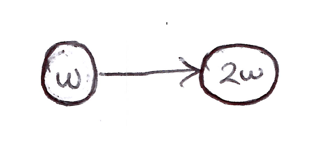
Simple Counterexample: 2-state part of an MDP.
- $w$ updates will diverge to infinity, since the transition will always look good (higher next-state estimated value than current state estimated value).
- The TD error on a transition between the 2 states is:
- The off-policy, semi-gradient TD(0) update is:
Example 2 (Baird’s Counterexample)
- Now let’s look at an entire complete system with instability (divergence).
- Consider the episodic 7-state, 2-action MDP shown below.
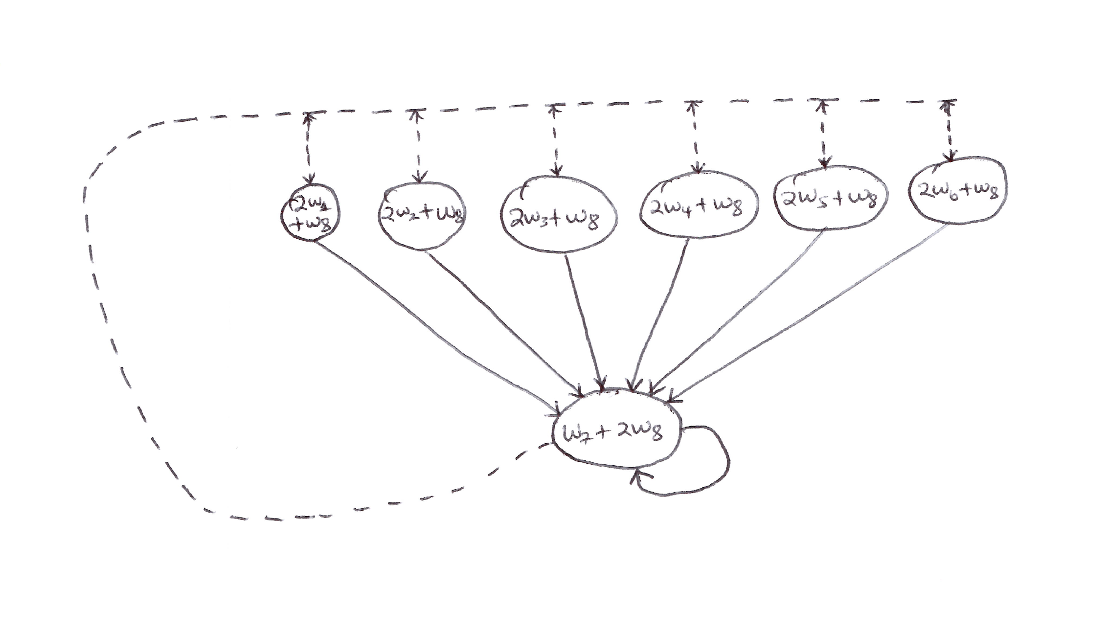
Baird’s Counterexample: Episodic 7-state, 2-action MDP.
- Assumptions/knowns:
- $b(\text{dashed}\,\vert\,\cdot) = 6/7$
- $b(\text{solid}\,\vert\,\cdot) = 1/7$
- $\pi(a\,\vert\,\cdot) = \pi(\text{solid}\,\vert\,\cdot) = 1$
- $R = 0$ (on all transitions)
- $\gamma = 0.99$
- The state values are estimated via linear parametrization.
- The estimated value of the leftmost state is $2w_1 + w_8$, which corresponds to a feature vector for the 1st state being:
- Since there are 8 components of the weight vector (more than the 7 non-terminal states), there exist many solutions.
- Applying semi-gradient TD(0) to this problem will cause the weights to diverge to infinity. This also applies for the dynamic programming (DP) case.
- The semi-gradient DP update is:
- This example shows that even the simplest combination of bootstrapping and function approximation can be unstable in the off-policy case.
- Simplest bootstrapping: DP and TD.
- Simplest function approximation: linear, semi-gradient descent method.
Example 3 (Tsitsiklis & Van Roy’s Counterexample)
This extends Example 1 with a terminal state and $R = 0$:
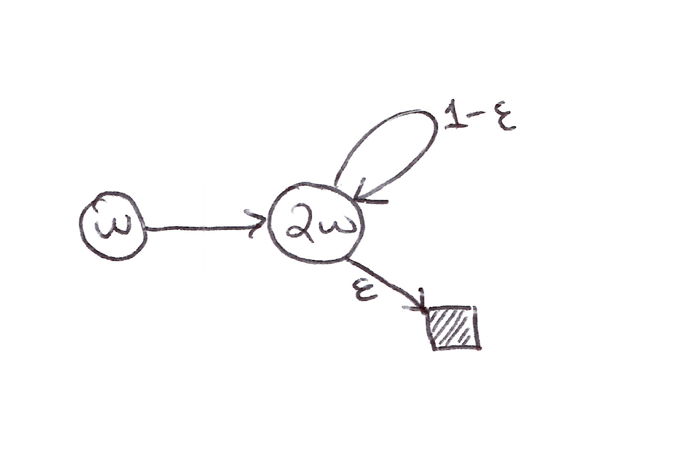
Tsitsiklis & Van Roy’s Counterexample: Extension of Example 1 with probability $\varepsilon$ of transitioning to the terminal state (shaded).
- Let’s find $w_{k+1}$ at each step that minimizes the $\overline{\text{VE}}$ between the estimated value and the expected one-step return:
- The sequence ${w_k}$ diverges when $\gamma > \dfrac{5}{6 - 4\varepsilon}$ and $w_0 \neq 0$.
Takeaways
- Instability can be prevented by using special methods for function approximation.
- These special methods guarantee stability because they do not extrapolate from the observed targets. They are called averagers.
- Averagers include:
- Nearest neighbor
- Locally weighted regression
- Tile coding
- Artificial neural networks (ANNs)
11.3 The Deadly Triad
- The danger of instability and divergence arises when we combine these 3 elements, which make up the deadly triad:
- Function approximation
- Bootstrapping
- Off-policy training
- Instability can be avoided if one of the elements is absent:
- Function approximation cannot be given up (needed for large-scale problems).
- Bootstrapping can be given up but at the cost of computational and data efficiency.
- Off-policy can be given up (replace Q-learning with Sarsa).
- There is no perfect solution as we still need off-policy for planning and parallel learning.
11.4 Linear Value-Function Geometry
- To better understand the stability challenge of off-policy learning, let’s think about value-function approximation more abstractly and independently of how learning is done.
- Let’s consider the case with 3 states $S = {s_1, s_2, s_3}$ and 2 parameters $\mathbf{w} = (w_1, w_2)^T$.
- All value functions exist in a 3-D space, however the parameters provide a 2-D subspace.
- Any weight vector $\mathbf{w} = (w_1, w_2)^T$ is a point in the 2-D subspace and thus also a complete value function $v_\mathbf{w}$ that assigns values to all 3 states.
- In linear value-function approximation, the subspace is a simple plane.
- How do we represent $v_\pi$ in the $d$-dimensional space?
- We need to perform a projection operation.
- TD methods present other solutions.
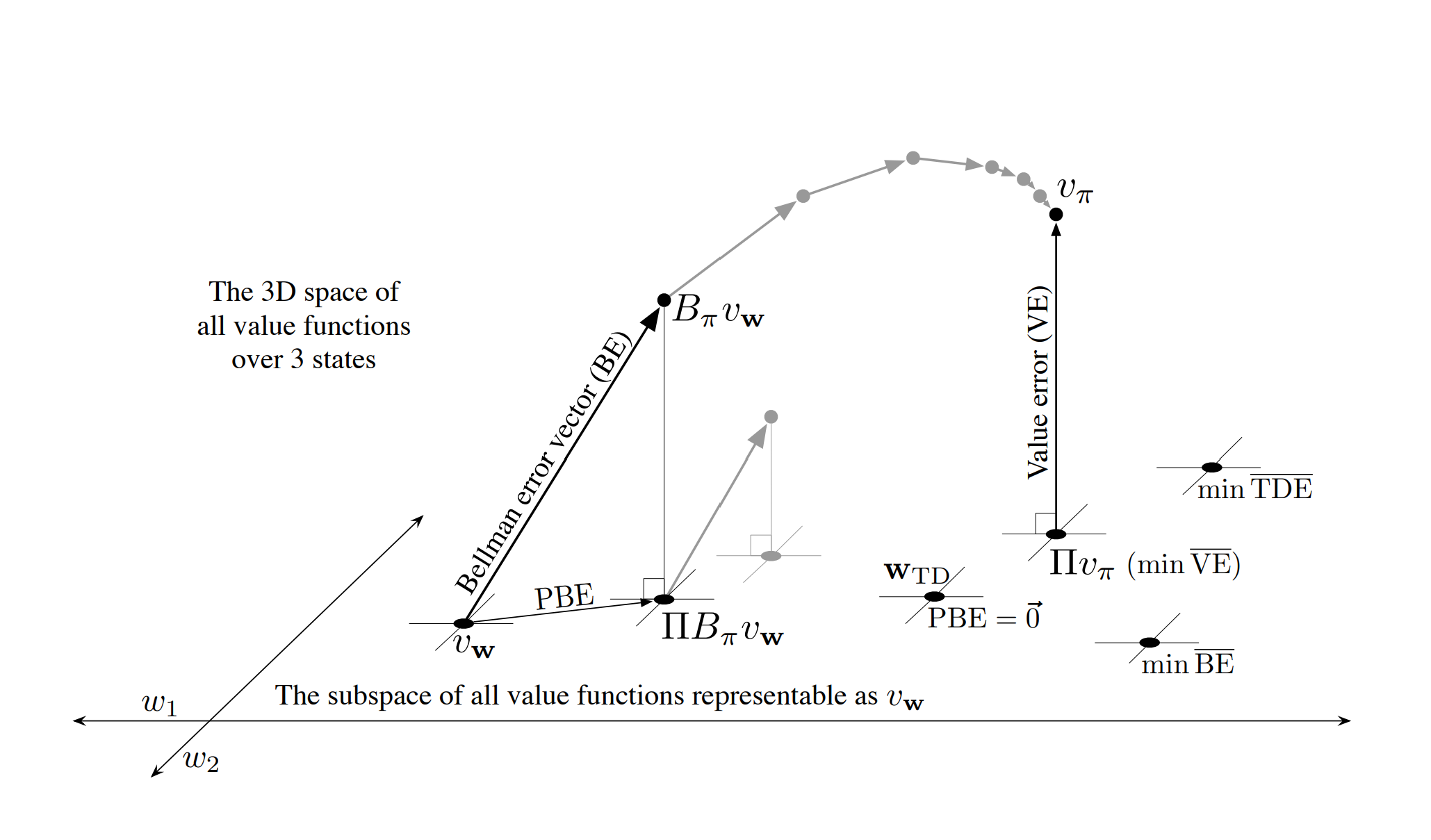
Shown is the 3D space of all value functions over three states, while shown as a plane is the subspace of all value functions representable by a linear function approximator with parameter $\mathbf{w} = (w_1, w_2)^T$. The true value function $v_\pi$ is in the larger space and can be projected down (into the subspace, using a projection operator $\Pi$) to its best approximation in the value error ($\text{VE}$) sense. The best approximators in the Bellman error ($\text{BE}$), projected Bellman error ($\text{PBE}$), and temporal difference error ($\text{TDE}$) senses are all potentially different and are shown in the lower right.
Projection Operation
- For the projection operation, the distance between value functions using the norm is:
-
The representable value function that is closest to the true value function $V_\pi$ is its projection $\Pi V_\pi$ (MC method asymptotic solution).
-
Projection matrix: with $\mathbf{D} \equiv \vert S \vert \times \vert S \vert$ diagonal matrix with $\mu(s)$ on the diagonal and $\mathbf{X} \equiv \vert S \vert \times d$ matrix whose rows are the feature vectors $\mathbf{x}(s)^T$:
\[\Pi \doteq \mathbf{X}\!\left(\mathbf{X}^T \mathbf{D} \mathbf{X}\right)^{-1} \mathbf{X}^T \mathbf{D}\]If the inverse does not exist, the pseudoinverse is substituted. Using these matrices, the squared norm of a vector can be written as:
\[\lVert v \rVert_\mu^2 = v^T \mathbf{D}\, v\]and the approximate linear value function written as:
\[v_\mathbf{w} = \mathbf{X}\mathbf{w}\]
TD Solutions
Bellman Error
- The true value function $v_\pi$ solves the Bellman equation exactly.
- The Bellman error shows how far off $v_\mathbf{w}$ is from $v_\pi$. The Bellman error at state $s$ is:
- The Bellman error is the expectation of the TD error.
- The vector of all the Bellman errors, at all states, $\bar{\delta}_\mathbf{w} \in \mathbb{R}^{\vert S \vert}$, is called the Bellman error vector ($\text{BE}$).
- The overall size of $\text{BE}$ is the Mean Squared Bellman Error, $\overline{\text{BE}}$:
- The Bellman operator $B_\pi : \mathbb{R}^{\vert S \vert} \to \mathbb{R}^{\vert S \vert}$ is defined by:
- The projection of the Bellman error vector back into the representable space creates the Projected Bellman Error $(\text{PBE})$ vector:
- The size of $\text{PBE}$, in the norm, is another measure of error in the approximate value function, called the Mean Square Projected Bellman Error, $\overline{\text{PBE}}$:
- With linear function approximation, there always exists an approximate value function (within the subspace) with zero $\overline{\text{PBE}}$; this is the TD fixed point $\mathbf{w}_\text{TD}$.
11.5 Gradient Descent in the Bellman Error
- Let’s apply the approach of SGD in dealing with the challenge of stability in off-policy learning.
TD Error (Naive Residual-Gradient Algorithm)
- Let’s take the minimization of the expected square of the TD error as the objective, TD(0):
- Using the TD error, we can find the Mean Squared TD error, the objective function $\overline{\text{TDE}}$:
- Following the standard SGD approach, the per-step update based on a sample of this expected value:
- This is the same as the semi-gradient TD algorithm except for the additional final term.
- This method is naive because it achieves temporal smoothing-like behavior rather than accurate prediction by penalizing all TD errors.
Bellman Error (Residual-Gradient Algorithm)
- Consider the minimization of the Bellman error (if the exact values are learned, the Bellman error is zero everywhere).
-
This yields the residual gradient algorithm:
\[\begin{align*} \mathbf{w}_{t+1} &= \mathbf{w}_t - \tfrac{1}{2}\alpha \nabla\!\left(\mathbb{E}_\pi\!\left[\delta_t\right]^2\right) \\ &= \mathbf{w}_t - \tfrac{1}{2}\alpha \nabla\!\left(\mathbb{E}_b\!\left[\rho_t\, \delta_t\right]^2\right) \\ &= \mathbf{w}_t - \alpha\, \mathbb{E}_b\!\left[\rho_t\, \delta_t\right] \nabla \mathbb{E}_b\!\left[\rho_t\, \delta_t\right] \\ &= \mathbf{w}_t - \alpha\, \mathbb{E}_b\!\left[\rho_t\!\left(R_{t+1} + \gamma \hat{v}(S_{t+1}, \mathbf{w}) - \hat{v}(S_t, \mathbf{w})\right)\right] \mathbb{E}_b\!\left[\rho_t \nabla \delta_t\right] \\ &= \mathbf{w}_t + \alpha\!\left[\mathbb{E}_b\!\left[\rho_t\!\left(R_{t+1} + \gamma \hat{v}(S_{t+1}, \mathbf{w})\right)\right] - \hat{v}(S_t, \mathbf{w})\right]\!\left[\nabla \hat{v}(S_t, \mathbf{w}) - \gamma\, \mathbb{E}_b\!\left[\rho_t \nabla \hat{v}(S_{t+1}, \mathbf{w})\right]\right] \end{align*}\] - Two ways to make the residual-gradient algorithm work:
- In the case of deterministic environments.
- Obtain 2 independent samples of the next state $S_{t+1}$ from $S_t$.
-
In both ways above, the algorithm is guaranteed to converge to a minimum of the $\overline{\text{BE}}$ under the usual conditions on the step-size parameter.
- However, there are at least 3 ways in which the convergence of the residual-gradient algorithm is unsatisfactory:
- Very slow.
- Converges to the wrong values.
- A problem with the $\overline{\text{BE}}$ objective covered in the next section.
11.6 The Bellman Error is Not Learnable
- The Bellman error is not learnable from the observed sequence of feature vectors, actions, and rewards.
- Since the Bellman error objective cannot be learned from the observable data, this is the strongest reason not to seek it.
- Examples of non-learnable Markov Reward Processes (MRPs):
Example 1

Value Error (VE) Learnability Counterexample: Deterministic MRP pair with an endless stream of $0$s and $2$s
- These MRPs have a deterministic reward with observable data of an endless stream of 0s and 2s.
- We cannot learn if the MRP has one state or two, or is stochastic or deterministic.
- The pair of MRPs shows that the $\overline{\text{VE}}$ objective is not learnable:
- The $\overline{\text{VE}}$ is not learnable, but the parameter that optimizes it is!
- We introduce a learnable natural objective function that is always observable. This is the error between the value estimate at each time and the return from that time, called the return error. The Mean Square Return Error $(\overline{\text{RE}})$ is the expectation, under $\mu$, of the square of this return error.
- $\overline{\text{RE}}$ in the on-policy case is:
- The $\overline{\text{BE}}$ can be computed from knowledge of the MDP but is not learnable from data, and its minimum solution is not learnable.
Example 2
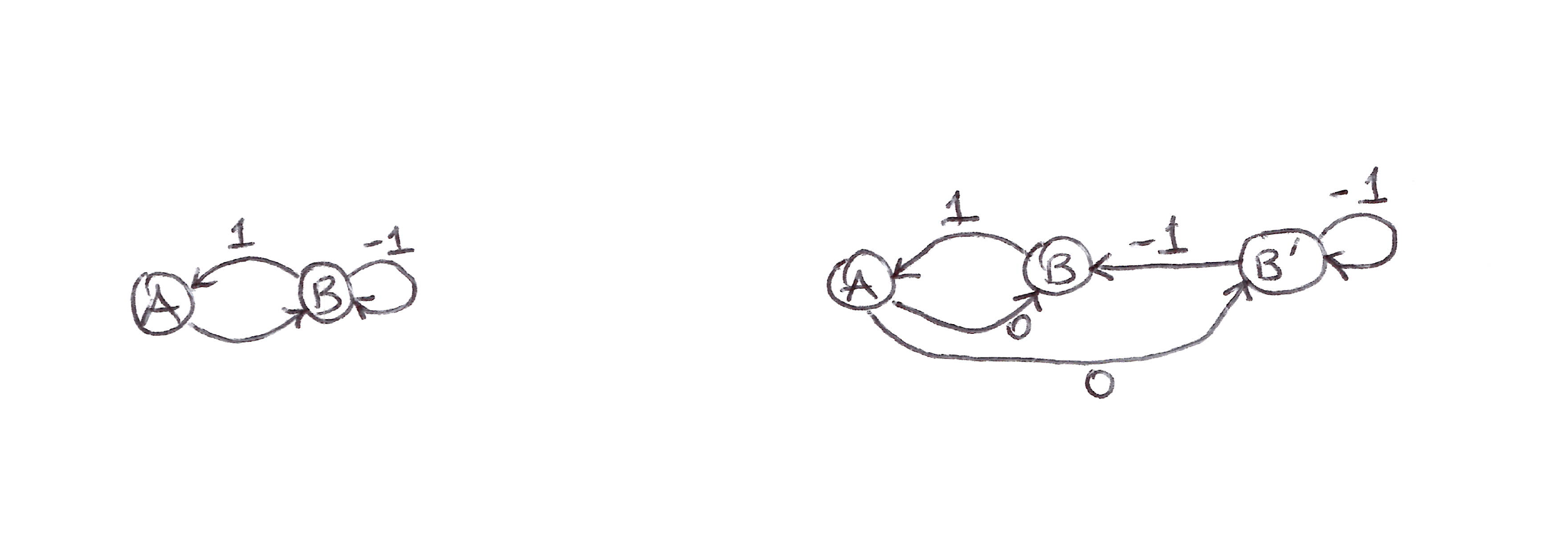
Bellman Error (BE) Learnability Counterexample: Complex Deterministic MRP pair with same distribution but different minimizing parameter vector
- The example above serves as a counterexample to the learnability of the Bellman error.
- The 2 MRPs generate the same data distribution but have different minimizing parameter vectors, proving that the optimal parameter vector is not a function of the data and thus cannot be learned from it.
- Other bootstrapping objectives, like $\overline{\text{PBE}}$ and $\overline{\text{TDE}}$, are learnable from data and yield optimal solutions different from each other and that of $\overline{\text{BE}}$.
- $\overline{\text{BE}}$ is limited to model-based settings, therefore $\overline{\text{PBE}}$ is preferred.
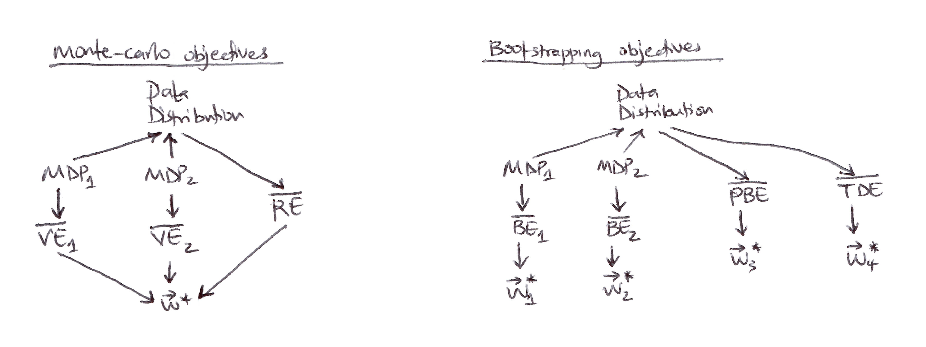
Left, Monte Carlo objectives: Two different MDPs can produce the same data distribution yet also produce different $\overline{\text{VE}}$s, proving that the $\overline{\text{VE}}$ objective cannot be determined from data and is not learnable. However, all such $\overline{\text{VE}}$s must have the same optimal parameter vector, $\mathbf{w}^{*}$! Moreover, this same $\mathbf{w}^{*}$ can be determined from another objective, the $\overline{\text{RE}}$, which is uniquely determined from the data distribution. Thus $\mathbf{w}^{*}$ and the $\overline{\text{RE}}$ are learnable even though the $\overline{\text{VE}}$s are not.
Right, Bootstrapping objectives: Two different MDPs can produce the same data distribution yet also produce different $\overline{\text{BE}}$s and have different minimizing parameter vectors; these are not learnable from the data distribution. The $\overline{\text{PBE}}$ and $\overline{\text{TDE}}$ objectives and their (different) minima can be directly determined from data and thus are learnable.
11.7 Gradient-TD Methods
- Let’s consider SGD methods for minimizing the $\overline{\text{PBE}}$.
- True SGD methods, Gradient-TD methods, have robust convergence properties even under off-policy training and nonlinear function approximation.
- In the linear case, there exists an exact solution, the TD fixed point $\mathbf{w}_\text{TD}$, at which the $\overline{\text{PBE}}$ is zero.
- This solution via least-squares methods yields a $O(d^2)$ complexity; however, we want an SGD method with $O(d)$ that converges robustly.
-
Let’s derive an SGD method for the $\overline{\text{PBE}}$ assuming linear function approximation:
\[\begin{align*} \overline{\text{PBE}}(\mathbf{w}) &= \lVert \Pi\, \bar{\delta}_\mathbf{w} \rVert_\mu^2 \\ &= \left(\Pi\, \bar{\delta}_\mathbf{w}\right)^T \mathbf{D}\, \Pi\, \bar{\delta}_\mathbf{w} \\ &= \bar{\delta}_\mathbf{w}^T \Pi^T \mathbf{D}\, \Pi\, \bar{\delta}_\mathbf{w} \\ &= \bar{\delta}_\mathbf{w}^T \mathbf{D} \mathbf{X}\!\left(\mathbf{X}^T \mathbf{D} \mathbf{X}\right)^{-1} \mathbf{X}^T \mathbf{D}\, \bar{\delta}_\mathbf{w} \\ &= \left(\mathbf{X}^T \mathbf{D}\, \bar{\delta}_\mathbf{w}\right)^T \!\left(\mathbf{X}^T \mathbf{D} \mathbf{X}\right)^{-1} \!\left(\mathbf{X}^T \mathbf{D}\, \bar{\delta}_\mathbf{w}\right) \end{align*}\]$\quad \left(\text{using } \Pi = \mathbf{X}!\left(\mathbf{X}^T \mathbf{D} \mathbf{X}\right)^{-1} \mathbf{X}^T \mathbf{D} \text{ and the identity } \Pi^T \mathbf{D} \Pi = \mathbf{D} \mathbf{X}!\left(\mathbf{X}^T \mathbf{D} \mathbf{X}\right)^{-1} \mathbf{X}^T \mathbf{D}\right)$
- The gradient of the $\overline{\text{PBE}}$ w.r.t $\mathbf{w}$ is:
- Let’s turn this into an SGD method via converting the 3 factors above into expectations under this distribution:
Substituting these expectations for the three factors into $\nabla \overline{\text{PBE}}$:
\[\nabla \overline{\text{PBE}}(\mathbf{w}) = 2\, \mathbb{E}\!\left[\rho_t\!\left(\gamma \mathbf{x}_{t+1} - \mathbf{x}_t\right) \mathbf{x}_t^T\right] \mathbb{E}\!\left[\mathbf{x}_t\, \mathbf{x}_t^T\right]^{-1} \mathbb{E}\!\left[\rho_t\, \delta_t\, \mathbf{x}_t\right]\]- The 1st and last terms are not independent (biased gradient estimate).
- Could estimate all 3 terms separately and combine (unbiased gradient estimate) but too computationally expensive.
Gradient-TD
- Estimate and store the product of the last 2 terms of $\nabla \overline{\text{PBE}}(\mathbf{w})$ (product of a $d \times d$ matrix and a $d$-vector yields a $d$-vector like $\mathbf{w}$ itself):
- In linear supervised learning, this is the solution to a linear least-squares problem for $\rho_t\, \delta_t$ approximation from the features.
- The standard SGD method for incrementally finding $\mathbf{v}$ that minimizes the expected squared error $\left(\mathbf{v}^T \mathbf{x}_t - \rho_t\, \delta_t\right)^2$ is known as the Least Mean Square (LMS) rule:
GTD2
-
With $\mathbf{v}_t$, we can update $\mathbf{w}_t$ using SGD:
\[\begin{align*} \mathbf{w}_{t+1} &= \mathbf{w}_t - \tfrac{1}{2}\alpha \nabla \overline{\text{PBE}}(\mathbf{w}_t) \\ &= \mathbf{w}_t - \tfrac{1}{2}\alpha\!\left(2\, \mathbb{E}\!\left[\rho_t\!\left(\gamma \mathbf{x}_{t+1} - \mathbf{x}_t\right) \mathbf{x}_t^T\right] \mathbb{E}\!\left[\mathbf{x}_t\, \mathbf{x}_t^T\right]^{-1} \mathbb{E}\!\left[\rho_t\, \delta_t\, \mathbf{x}_t\right]\right) \\ &= \mathbf{w}_t + \alpha\, \mathbb{E}\!\left[\rho_t\!\left(\mathbf{x}_t - \gamma \mathbf{x}_{t+1}\right) \mathbf{x}_t^T\right] \mathbb{E}\!\left[\mathbf{x}_t\, \mathbf{x}_t^T\right]^{-1} \mathbb{E}\!\left[\rho_t\, \delta_t\, \mathbf{x}_t\right] \\ &\approx \mathbf{w}_t + \alpha\, \mathbb{E}\!\left[\rho_t\!\left(\mathbf{x}_t - \gamma \mathbf{x}_{t+1}\right) \mathbf{x}_t^T\right] \mathbf{v}_t \\ &\approx \mathbf{w}_t + \alpha \rho_t\!\left(\mathbf{x}_t - \gamma \mathbf{x}_{t+1}\right) \mathbf{x}_t^T \mathbf{v}_t \end{align*}\]where $O(d)$ per-step computational complexity of $(\mathbf{x}_t^T \mathbf{v}_t)$ is done first.
TD(0) with Gradient Correction (GTD(0) or TDC)
-
Let’s look at another analytical algorithm called TD(0) with gradient correction, TDC:
\[\begin{align*} \mathbf{w}_{t+1} &= \mathbf{w}_t + \alpha\, \mathbb{E}\!\left[\rho_t\!\left(\mathbf{x}_t - \gamma \mathbf{x}_{t+1}\right) \mathbf{x}_t^T\right] \mathbb{E}\!\left[\mathbf{x}_t\, \mathbf{x}_t^T\right]^{-1} \mathbb{E}\!\left[\rho_t\, \delta_t\, \mathbf{x}_t\right] \\ &= \mathbf{w}_t + \alpha\!\left(\mathbb{E}\!\left[\rho_t\, \mathbf{x}_t\, \mathbf{x}_t\right] - \gamma\, \mathbb{E}\!\left[\rho_t\, \mathbf{x}_{t+1}\, \mathbf{x}_t^T\right]\right) \mathbb{E}\!\left[\mathbf{x}_t\, \mathbf{x}_t^T\right]^{-1} \mathbb{E}\!\left[\rho_t\, \delta_t\, \mathbf{x}_t\right] \\ &= \mathbf{w}_t + \alpha\!\left(\mathbb{E}\!\left[\mathbf{x}_t\, \mathbf{x}_t\right] - \gamma\, \mathbb{E}\!\left[\rho_t\, \mathbf{x}_{t+1}\, \mathbf{x}_t^T\right]\right) \mathbb{E}\!\left[\mathbf{x}_t\, \mathbf{x}_t^T\right]^{-1} \mathbb{E}\!\left[\rho_t\, \delta_t\, \mathbf{x}_t\right] \\ &= \mathbf{w}_t + \alpha\!\left(\mathbb{E}\!\left[\mathbf{x}_t\, \rho_t\, \delta_t\right] - \gamma\, \mathbb{E}\!\left[\rho_t\, \mathbf{x}_{t+1}\, \mathbf{x}_t^T\right] \mathbb{E}\!\left[\mathbf{x}_t\, \mathbf{x}_t^T\right]^{-1} \mathbb{E}\!\left[\rho_t\, \delta_t\, \mathbf{x}_t\right]\right) \\ &\approx \mathbf{w}_t + \alpha\!\left(\mathbb{E}\!\left[\mathbf{x}_t\, \rho_t\, \delta_t\right] - \gamma\, \mathbb{E}\!\left[\rho_t\, \mathbf{x}_{t+1}\, \mathbf{x}_t^T\right] \mathbf{v}_t\right) \\ &\approx \mathbf{w}_t + \alpha \rho_t\!\left(\delta_t\, \mathbf{x}_t - \gamma \mathbf{x}_{t+1}\, \mathbf{x}_t^T \mathbf{v}_t\right) \end{align*}\]with $O(d)$ complexity if the final product $(\mathbf{x}_t^T \mathbf{v}_t)$ is done first.
Takeaways
- GTD2 and TDC both involve 2 learning processes: a primary one for $\mathbf{w}$ and a secondary one for $\mathbf{v}$.
- Asymmetrical dependence ($\mathbf{w}$ depends on $\mathbf{v}$ but $\mathbf{v}$ does not depend on $\mathbf{w}$) is referred to as a cascade.
- Gradient-TD methods are the most well-understood and widely used stable off-policy methods.
- Extensions of GTD methods include to:
- Action values and control: GQ [Maei et al., 2010]
- Eligibility traces: GTD($\lambda$), GQ($\lambda$) [Maei, 2011; Maei & Sutton, 2010]
- Nonlinear function approximation [Maei et al., 2009]
- Hybrid algorithms include:
- Midway between semi-gradient TD and gradient TD [Hackman, 2012; White & White, 2016]
- GTD + proximal methods & control variates [Mahadevan et al., 2014; Du et al., 2017]
11.8 Emphatic-TD Methods
- Let’s explore a major strategy for obtaining a cheap and efficient off-policy learning method with function approximation.
- Recall that linear semi-gradient TD methods are stable when trained under the on-policy distribution .
- The match between the on-policy state distribution $\mu_\pi$ and the state-transition probabilities $p(s’ \vert s, a)$ under the target policy does not exist in off-policy learning.
- Mismatch Fix:
- Re-weight the states, emphasizing some and de-emphasizing others, so as to return the distribution of the updates to the on-policy distribution.
- Then there would be a match, and convergence and stability would be achieved. This is the idea of Emphatic-TD methods.
- The one-step Emphatic-TD algorithm for learning episodic state values is defined by:
- Applying Emphatic TD to Baird’s counterexample yields very high variance results (impossible to get consistent results in experiments).
- We focus on how we reduce the variance in all these algorithms in the next section.
11.9 Reducing Variance
- Off-policy learning is inherently of greater variance than on-policy learning.
- The raison d’être of off-policy learning is to enable generalization to the vast number of related-but-not-identical policies.
- Why is variance control critical in off-policy learning based on importance sampling?
- Recall importance sampling involves products of policy ratios:
- The policy ratios always have an expected value of 1, but their actual values might be high or as low as 0:
- Successive ratios are uncorrelated, so their products are always 1 in expected value, but they can be of high variance.
- These ratios multiply the step size in SGD methods, so their high variance is problematic for SGD because of the occasional huge steps.
- How can we alleviate the effects of high variance via small step-size settings enough to ensure the expected step taken by SGD is small? Some approaches:
- Momentum
- Polyak-Ruppert averaging
- Methods for adaptively setting separate step sizes for different components of the parameter vector
- “Importance weight aware” updates of Karampatziakis & Langford (2015)
- Weighted importance sampling, which is well-behaved with lower variance updates than ordinary importance sampling, but adapting it to function approximation is challenging [Mahmood & Sutton, 2015]
- Tree backup algorithm (off-policy, without importance sampling)
- Allow the target policy $\pi$ to be determined partly by the behavior policy $b$ to limit creating large importance sampling ratios
11.10 Summary
- Off-policy learning poses a challenge that requires creating stable and efficient learning algorithms.
- Tabular Q-learning makes off-policy learning seem easy, as does its generalizations to Expected Sarsa and tree backup.
- Extension further to function approximation (even linear) is challenging.
- The challenge of off-policy learning is divided into two parts:
- Correcting the targets of learning for the behavior policy.
- Dealing with the instability of bootstrapping (mismatch between off-policy and on-policy distribution of updates).
- The deadly triad arises when we try to combine these 3 elements: function approximation, off-policy learning, and bootstrapping, thereby causing instability and divergence.
- SGD in the Bellman error $\overline{\text{BE}}$ is not learnable so it does not work.
- Gradient-TD methods perform SGD in the projected Bellman error $\overline{\text{PBE}}$ and are learnable with $O(d)$ computational complexity.
- Emphatic-TD methods re-weight updates, emphasizing some and de-emphasizing others, to get the off-policy distribution of the updates to match that of on-policy.
- There are many ways of reducing high variance in off-policy learning that are centered on minimizing the step taken by SGD by using small step-size parameters to counter the multiplicative effect from the successive policy ratios.
Citation
If you found this blog post helpful, please consider citing it:
@article{obasi2026RLsuttonBartoCh11notes,
  title   = "Sutton & Barto, Ch. 11: Off-Policy Methods with Approximation (Personal Notes)",
  author  = "Obasi, Chizoba",
  journal = "chizkidd.github.io",
  year    = "2026",
  month   = "Mar",
  url     = "https://chizkidd.github.io/2026/03/09/rl-sutton-barto-notes-ch011/"
}