Sutton & Barto, Ch. 09: On-Policy Prediction with Approximation (Personal Notes)
- Study of function approximation in RL by considering its use in estimating the state-value function from on-policy data, i.e. in approximating $v_\pi$ from experience generated using a known policy $\pi$.
- The approximate value function is represented as a parameterized functional form with weight vector $\mathbf{w} \in \mathbb{R}^d$:
- The function above is for the approximate value of state $s$ given weight vector $\mathbf{w}$.
- $\hat{v}$ might be a linear function, a multi-layer artificial neural network, or a decision tree.
- Extending RL to function approximation makes it applicable to partially observable problems, in which the full state is unavailable to the agent.
- Function approximation cannot augment the state representation with memories of past observations.
Table of Contents
- 9.1 Value-Function Approximation
- 9.2 The Prediction Objective (VE)
- 9.3 Stochastic-Gradient & Semi-Gradient Methods
- 9.4 Linear Methods
- 9.5 Feature Construction for Linear Methods
- 9.6 Selecting Step-Size Parameters Manually
- 9.7 Nonlinear Function Approximation: Artificial Neural Networks (ANNs)
- 9.8 Least-Squares TD (LSTD)
- 9.9 Memory-based Function Approximation
- 9.10 Kernel-based Function Approximation
- 9.11 Looking Deeper at On-Policy Learning: Interest & Emphasis
- 9.12 Summary
Appendix
9.1 Value-Function Approximation
- All the prediction methods covered so far involve an update to an estimated value function that shifts its value towards a “backed-up value” (update target, $u$). Let’s denote an individual state update by $s \mapsto u$:
- Each update is interpretable as an example of the desired input-output behaviour of the value function.
- Until now, the value function updates have been made in the tabular setting, which is quite trivial because estimated values of all other states are left unchanged.
- Now using arbitrarily complex and sophisticated methods to perform the update, updating at $s$ generalizes so that the estimated value of many other states are changed as well.
- Machine learning methods that learn to mimic input-output examples in this way are called supervised learning methods, and when the outputs are numbers, like $u$, the process is called function approximation.
- Function approximation methods expect to receive examples of the desired input-output behavior of the function they are trying to approximate.
- We view each update as a conventional training example.
- This allows us to use any of a wide range of existing function approximation methods for value prediction.
- Whatever function approximation method is chosen needs to be able to perform online learning.
9.2 The Prediction Objective ($\overline{\text{VE}}$)
- We have more states $s$ than weights $\mathbf{w}$, therefore we cannot feasibly approximate the value function perfectly.
- Making one state’s estimate more accurate invariably leads to making the others’ less accurate.
- Therefore, it is necessary to define which states we care most about, based on a state distribution, $\mu(s)$, that represents how much we care about the error in each state $s$.
- Weighting the error in a state $s$, the difference between the approximate value $\hat{v}(s, \mathbf{w})$ and the true value $v_\pi(s)$, over the state space by $\mu$ leads to obtaining a natural objective function called the mean squared value error, denoted by $\overline{\text{VE}}$:
- $\sqrt{\overline{\text{VE}}}$ tells us roughly how much the approximate values differ from the true values.
- Often $\mu$ is chosen to be the fraction of time spent in $s$, called the on-policy distribution under on-policy training.
On-policy Distribution
-
Continuing tasks: the on-policy distribution is the stationary distribution under $\pi$:
$$\mu(s) = \sum_{s'} \mu(s') \sum_a \pi(a \vert s')\, p(s \vert s', a), \quad \forall s \in S$$
$$
\begin{aligned}
\text{where} \\
\mu(s) &= \text{stationary probability of being in state } s \text{ under } \pi \\
s' &= \text{preceding state}
\end{aligned}
$$
Balance Equation
The probability of being in state $s$ equals the sum over all ways of arriving in $s$ from any previous state $s’$ under policy $\pi$.
-
Episodic tasks: it depends on how the initial states of episodes are chosen:
$$\eta(s) = h(s) + \sum_{\bar{s}} \eta(\bar{s}) \sum_a \pi(a \vert \bar{s})\, p(s \vert \bar{s}, a), \quad \forall s \in S$$
$$
\begin{aligned}
\text{where} \\
h(s) &= \text{probability that an episode begins in each state } s \\
\eta(s) &= \text{number of time steps spent, on average, in state } s \text{ in a single episode} \\
\bar{s} &= \text{preceding state}
\end{aligned}
$$
Visitation Equation
The expected number of visits to state $s$ equals the probability of starting in state $s$ plus the expected number of visits to all preceding states $s’$ that transition into $s$ under policy $\pi$.
- This system of equations can be solved for the expected number of visits $\eta(s)$.
- The on-policy distribution is the fraction of time spent in each state, normalized to sum to 1:
- If discounting exists, then we redefine $\eta(s)$:
Performance Objective
- Although $\overline{\text{VE}}$ is a good starting point, it’s not completely clear that it is the right performance objective.
- The ultimate goal (reason for learning a value function) is to find a better policy.
- If we use $\overline{\text{VE}}$, the goal is to find a global optimum (optimal weight vector, $\mathbf{w}^*$):
- Complex function approximators may converge to a local optimum:
9.3 Stochastic-Gradient & Semi-Gradient Methods
Stochastic Gradient Descent (SGD)
- SGD methods are among the most widely used of all function approximation methods and are well suited to online RL.
- The function approximator is parameterized by a weight vector with a fixed number of real components (column vector):
- In SGD, we update the weight vector at each time step by moving it in the direction that minimises the error most quickly for the example shown:
- The equation for $\nabla f(\mathbf{w})$, the gradient of $f$ WRT $\mathbf{w}$, is:
- SGD methods are “gradient descent” methods because the overall step in $\mathbf{w}_t$ is proportional to the negative gradient of the example’s squared error ($w_{t+1}$). This is the direction in which the error falls most rapidly.
- Gradient descent methods are called “stochastic” because the update is done on only a single example, which might have been selected stochastically.
- If $\alpha$ decreases as expected in satisfaction of the standard stochastic approximation conditions, then SGD is guaranteed to converge to a local optimum.
True Value Estimates
- When the true value function $v_\pi(S_t)$ is unknown, we can approximate it by substituting $U_t$ in place of $v_\pi(S_t)$.
- This yields the following general SGD method for state-value prediction:
- If $U_t$ is an unbiased estimate, that is, if \(\mathbb{E}[U_t \vert S_t = s] = v_\pi(s)\) for each $t$, then $\mathbf{w}_t$ is guaranteed to converge to a local optimum under the usual stochastic approximation conditions for decreasing $\alpha$.
- An example of an unbiased estimator is the Monte Carlo estimate for state $S_t$:
- Bootstrapping methods are biased in that their target is dependent on the current value of the weights $\mathbf{w}$.
- Semi-gradient (bootstrapping) methods converge reliably in linear cases.
- Bootstrapping targets could be $n$-step returns or dynamic programming (DP) targets.
State Aggregation
- A simple form of generalizing function approximation in which states are grouped together, with one estimated value (one component of the weight vector $\mathbf{w}$) for each group.
- A special SGD case in which:
9.4 Linear Methods
- One of the simplest cases for function approximation is when the approximate value function is a linear combination of the weight vector.
- Linear methods approximate the state-value function by the inner product between $\mathbf{w}$ and $\mathbf{x}(s)$:
- For linear methods, features are basis functions because they form a linear basis for the set of approximate functions.
- For linear methods, the gradient of the approximate value function WRT $\mathbf{w}$ is:
- Thus in the linear case, the general SGD update reduces to:
- The semi-gradient TD(0) algorithm converges under linear function approximation:
- Once the system has reached steady state, for any given $\mathbf{w}_t$ the expected next weight vector can be represented as:
- It is clear that, if the system converges, it must converge to the weight vector $\mathbf{w}_\text{TD}$ at which:
- $\mathbf{w}_\text{TD}$ is called the TD fixed point. It is the point that linear semi-gradient TD(0) converges to.
-
$\mathbf{A}$ needs to be positive definite to ensure that $\mathbf{A}^{-1}$ exists. \(y^T \mathbf{A} y > 0, \text{for any } y \neq 0\)
- The semi-gradient $n$-step TD algorithm is the natural extension of the tabular $n$-step TD algorithm in Ch. 7 to semi-gradient function approximation:
Bounded Expansion
- At the TD fixed point, $\overline{\text{VE}}$ is within a bounded expansion of the lowest possible error:
- That is, the asymptotic error of the TD method is no more than $\frac{1}{1-\gamma}$ times the smallest possible error (attained in the limit by the MC method).
- $\gamma$ is often near 1, so the expansion factor can be quite large; therefore there is substantial potential loss in asymptotic performance with the TD method.
- A bound analogous to TD’s fixed point & bound above on $\overline{\text{VE}}(\mathbf{w}_\text{TD})$ applies to other on-policy bootstrapping methods as well.
- One-step action-value methods such as semi-gradient Sarsa(0) converge to an analogous fixed point and an analogous bound.
- For episodic tasks, there exists a bound [Bertsekas & Tsitsiklis, 1996].
9.5 Feature Construction for Linear Methods
- Let’s discuss different ways of constructing features, which is important for function approximation in linear methods.
9.5.1 Polynomials
- There may be a need to design features with higher complexity that can be captured with linear methods.
- Say for example a state has 2 numerical dimensions, $s_1, s_2 \in \mathbb{R}$. Then it is insufficient to represent this state as $\mathbf{x}(s) = (s_1, s_2)^T$ because it does not take into account any interactions between the 2 dimensions.
- We can overcome this limitation by instead representing $s$ by the 4-D feature vector:
- For $k$ numerical dimensions, suppose each state $s$ corresponds to $k$ numbers, $s_1, s_2, s_3, \ldots, s_k \text{ with each } s_i \in \mathbb{R}$, each order-$n$ polynomial-basis feature $x_i$ can be written as:
9.5.2 Fourier Basis
- Fourier series express periodic functions as weighted sums of sine and cosine basis functions of different frequencies, with a function $f$ being periodic if:
- The 1-D, order-$n$ Fourier cosine basis consists of the $n+1$ features:
- For $k$-dimensional state space, the $i$-th feature in the order-$n$ Fourier cosine basis is:
9.5.3 Coarse Coding
- Mapping circles to the features of a state space for 2-dimension.
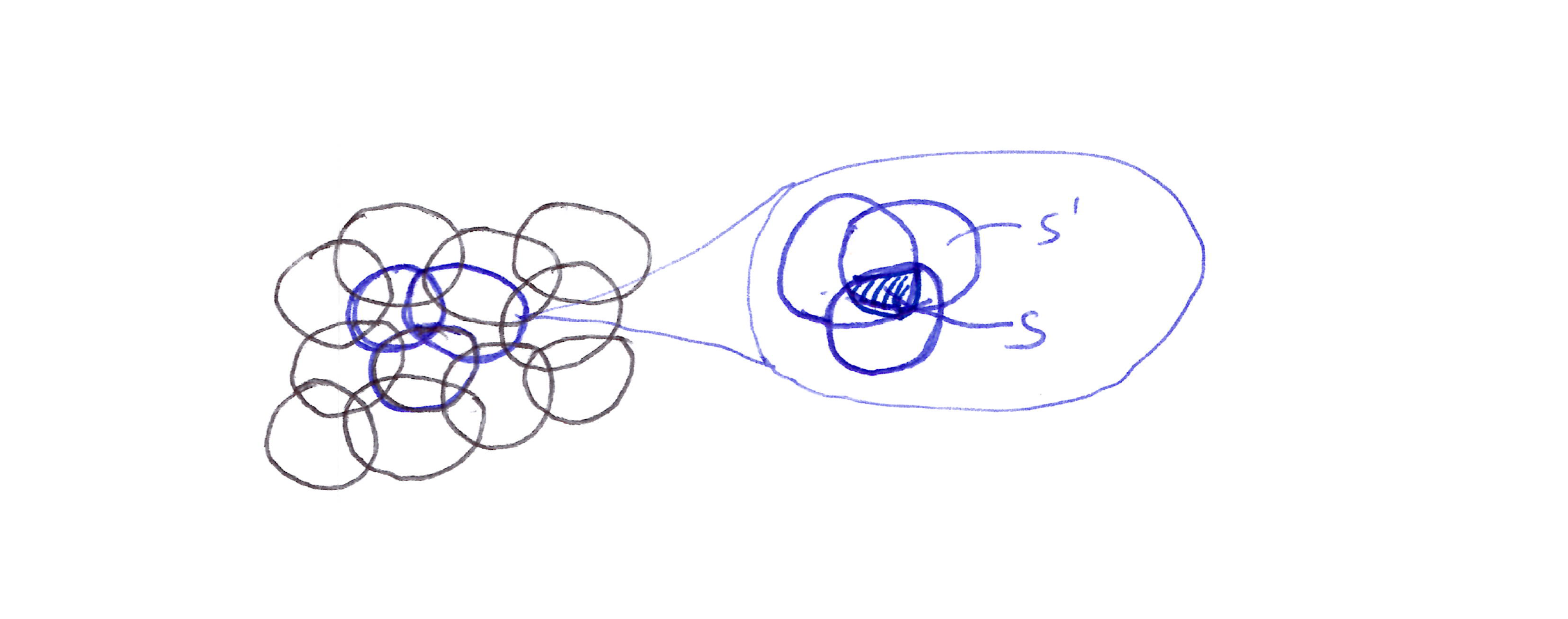
Generalization from state $s$ to state $s’$ depends on the number of their features whose receptive fields (in this case, circles) overlap. These states have one feature in common, so there will be slight generalization between them.
- In the diagram above, if the state is inside a circle, then the corresponding feature has the value of 1 and is said to be present; otherwise the feature is 0 and is said to be absent.
- This kind of 1-0 valued feature is called a binary feature.
- Representing a state with features that overlap in this way is known as coarse coding.
- If we train at one state (a point in the space), then the weights of all circles intersecting that state will be affected (each circle has a corresponding weight, a single $\mathbf{w}$ component).
- Generalization in linear function approximation methods is determined by the sizes and shapes of the features’ receptive fields.
9.5.4 Tile Coding
- Tile coding is a form of coarse coding for multi-dimensional continuous spaces that is flexible and computationally efficient.
- It may be the most practical feature representation for modern sequential digital computers.
- In tile coding, the receptive fields of the features are grouped into partitions of the state space.
- Each such partition is called a tiling, and each element of the partition is called a tile.
- These tiles can be sets that are overlapping, uniform, or asymmetrically distributed.
- The tiles do not need to be squares; they can be irregular shapes, horizontal/vertical/log lines.
- Advantages:
- Because tile coding works with partitions, the overall number of features that are active at one time is the same for any state.
- Because tile coding uses binary feature vectors, computing the approximate value function reduces to simply summing the $n$ weight components corresponding to the $n$ active tiles, rather than performing $d$ multiplications.
- Generalization extends to states sharing tiles with the trained state, proportional to tiles in common.
- Uniform offsets can introduce directional artifacts (e.g. diagonal bias);
- Asymmetric offsets produce better-centered patterns.
- Tilings are offset by $\frac{w}{n}$ (the fundamental unit).
- Uniform offsets use displacement vector $(1,1)$;
- Asymmetric offsets use $(1,3)$ for superior generalization.
- Miller & Glanz (1996) recommend displacement vectors of first odd integers $(1, 3, 5, \ldots, 2k-1)$ for $k$ dimensions, with $n$ set to a power of 2 $\geq 4k$.
- Tile number & size determine resolution, while tile shape determines generalization.
- Square tiles generalize equally
- Elongated tiles generalize along their longer dimension
- Diagonal tiles generalize along a diagonal.
- Mixed tile shapes (horizontal, vertical, conjunctive) allow per-dimension generalization while still learning values for specific conjunctions. Tile choice fully determines generalization behavior.
- Hashing pseudorandomly collapses a large tiling into a much smaller set of tiles (each consisting of noncontiguous, disjoint regions), drastically reducing memory requirements with little performance loss.
- This sidesteps the curse of dimensionality since memory need only match the task’s real demands rather than grow exponentially with dimensions.
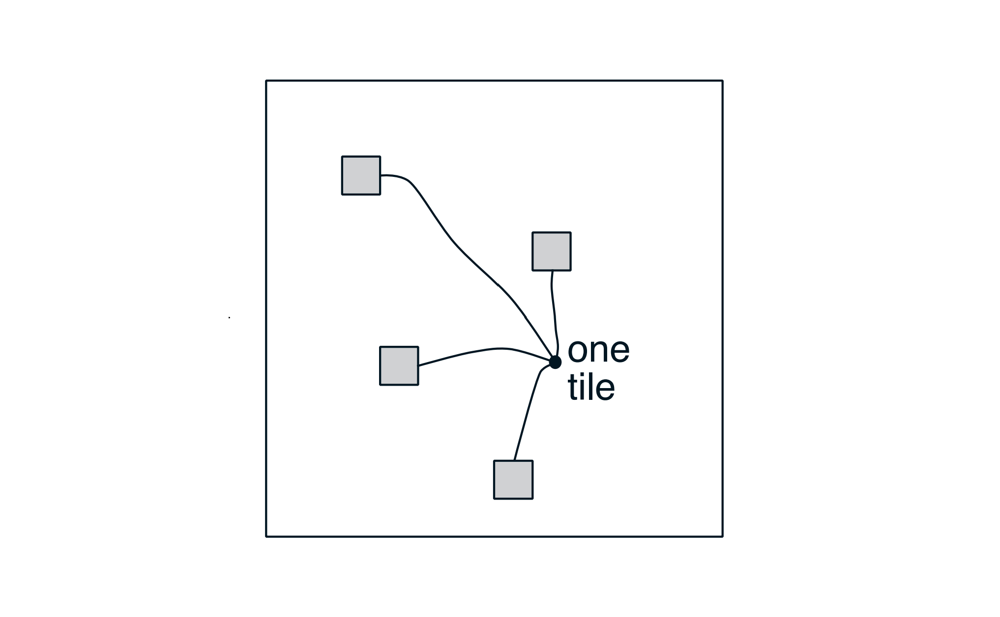
4 subtiles collapse into 1 tile in the above diagram.
9.5.5 Radial Basis Functions (RBF)
- RBFs are the natural extension/generalization of coarse coding to continuous-valued domain/feature space.
- Rather than a feature being 0 or 1 (binary), it can take any value in the interval $[0, 1]$.
- A typical RBF feature, $x_i$, has a Gaussian (bell-shaped) response $x_i(s)$ dependent only on the distance between the state $s$ and the feature’s center state $c_i$, and relative to the feature’s width $\sigma_i$:
- let’s see a 1-D example with a Euclidean distance metric
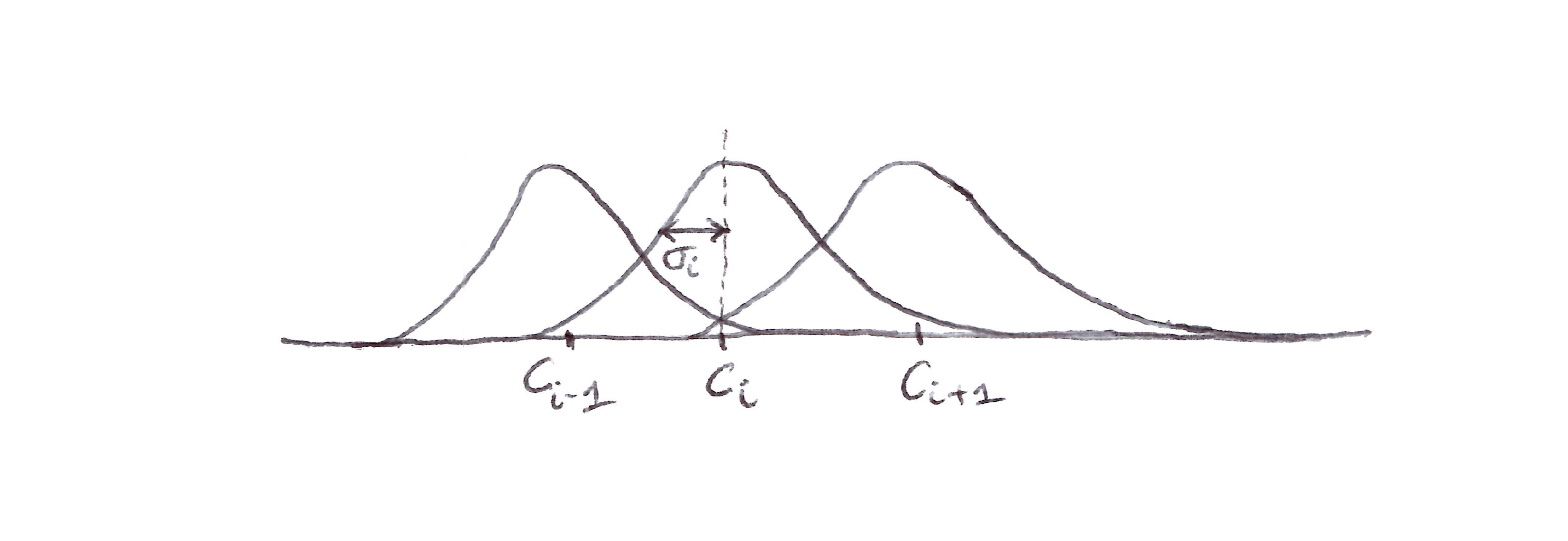
A one-dimensional example with a Euclidean distance metric.
- RBFs are more advantageous to binary features: they produce approximate functions that vary smoothly and are differentiable.
- An RBF network is a linear function approximator using RBFs for its features.
- Some learning methods for RBF networks change the features’ centers and widths, making them nonlinear function approximators.
- Nonlinear methods are much more precise in fitting the target functions, but (nonlinear) RBF networks are much more computationally complex and require more manual tuning before learning.
9.6 Selecting Step-Size Parameters Manually
- What is the best way to select $\alpha$ for function approximation?
- So far,
- The theory of stochastic approximation gives us conditions on a slowly decreasing step-size sequence that are sufficient to guarantee convergence, but these tend to result in learning that is too slow.
- The sample-average classical method $\alpha_t = \frac{1}{t}$ is not appropriate for TD methods, for nonstationary problems, or for any function approximation method.
- For linear methods, there are recursive least-square methods that set an optimal matrix step size which can be extended to LSTD methods (seen in Section 9.8), but these require $O(d^2)$ step-size parameters, or $d$ times more parameters than we are learning. Therefore, it is inappropriate for function approximation.
- A good rule of thumb for setting the step-size parameter of linear SGD models is:
- This rule of thumb works best if the feature vectors do not vary greatly in length; ideally $\mathbf{x}^T \mathbf{x}$ is a constant.
9.7 Nonlinear Function Approximation: Artificial Neural Networks (ANNs)
- ANNs are widely used for nonlinear function approximation.
- An ANN is a network of interconnected units that have some of the properties of neurons, the main components of nervous systems.
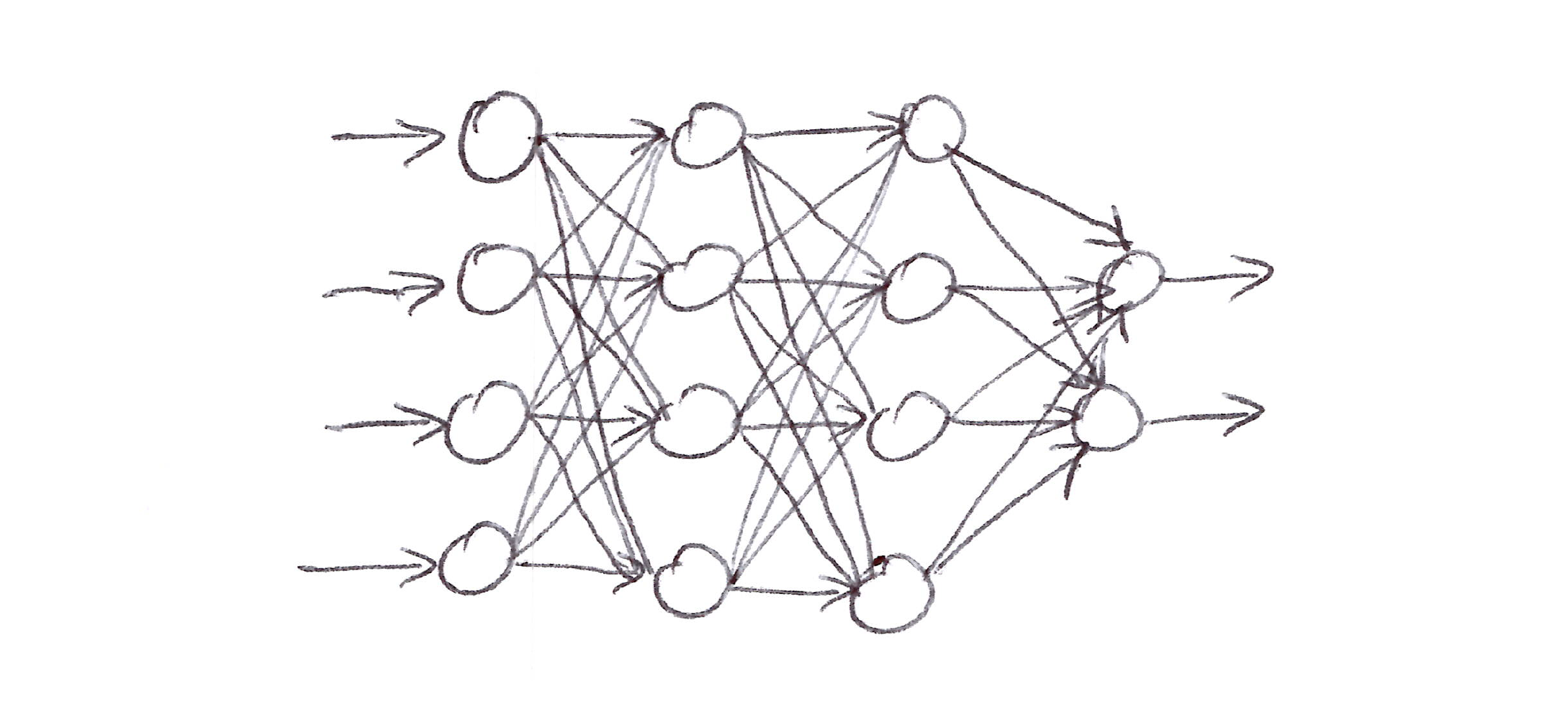
A generic feedforward Artifical Neural Network with 4 input units, 2 output units, and 2 hidden layers.
- The units (circles in the figure above) compute a weighted sum of their input signals, and then apply a nonlinear function, called the activation function, to the result.
-
Some activation functions include: \(\begin{aligned} \text{Sigmoid:} \quad & f(x) = \frac{1}{1 + e^{-x}} \\ \\ \text{ReLU:} \quad & f(x) = \max(0, x) \\ \\ \text{Binary step:} \quad & f(x) = \left\{ \begin{array}{ll} 1 & \text{if } x \geq 0 \\ 0 & \text{if } x < 0 \end{array} \right\} \end{aligned}\)
- ANNs can use TD errors to learn value functions, or they can aim to maximize expected reward as in a gradient bandit (Section 2.8) or a policy gradient algorithm (Chapter 13).
- Overfitting in ANNs is a problem for function approximation that can be reduced through the dropout method [Srivastava, Hinton, Krizhevsky, Sutskever & Salakhutdinov, 2014].
- Deep belief networks presented a major step towards solving the training problem of deep layers of a deep ANN [Hinton, Osindero & Teh, 2006].
- Batch normalization makes it easier to train deep ANNs by normalizing the output of deep layers before they feed into the following layer. This improves the learning rate of deep ANNs [Ioffe & Szegedy, 2015].
- Deep residual learning is another technique useful for training deep ANNs [He, Zhang, Ren & Sun, 2016].
- Deep Convolutional Networks have proven to be very successful in impressive RL algorithms [LeCun, Bottou, Bengio & Haffner, 1998].
- In summary, advances in the design and training of ANNs, of which we have only mentioned a few, all contribute to RL.
- Although current RL theory is mostly limited to methods using tabular or linear function approximation methods, the impressive performances of notable RL applications owe much of their success to nonlinear function approximation by multi-layer ANNs.
9.8 Least-Squares TD (LSTD)
- As established earlier, TD(0) with linear function approximator converges asymptotically (for appropriately decreasing step sizes) to the TD fixed point:
- Instead of computing $\mathbf{w}_\text{TD}$ iteratively, let’s compute estimates of $\mathbf{A}$ and $\mathbf{b}$ and then directly compute the TD fixed point. This is what Least-Squares TD (LSTD) does exactly. It forms the natural estimates:
- The LSTD estimated TD fixed point is:
Computational Complexity
- The inverse of $\mathbf{\hat{A}_t}$ computation costs $O(d^3)$, but this can be reduced to $O(d^2)$ using the Sherman-Morrison formula:
- LSTD does not require a step-size and as such means that it never forgets, which is sometimes desirable but often not in RL problems where both the policy and environment change with time.
- However in control applications, LSTD typically has to be combined with some other mechanism to induce forgetting, negating its advantage of not requiring a step-size parameter.
9.9 Memory-based Function Approximation
- So far we have been parametrising functions that approximate our value function, and these parameters are updated as we see more data. This is called the parametric approach.
- Memory-based function approximators store training examples in memory as they arrive without updating any parameters and retrieve them from memory upon query of a state value’s estimate.
- Memory-based function approximators are examples of non-parametric methods.
- Memory-based function approximation is sometimes called lazy learning because processing training examples is postponed until the system is queried to provide an output.
- Non-parametric methods could produce increasingly accurate approximations of any target function with increasing number of training examples accumulating in memory.
- There are different memory-based methods, but let’s focus on local learning:
- Local learning methods approximate a value function only locally in the neighborhood of the current query state by retrieving states in memory via a distance metric between the query state and training example states.
- Local learning methods discard the local approximation after the query state is assigned a value.
- Examples of local learning methods:
- Nearest Neighbor: retrieve from memory the closest state to the query state and return that example’s value as the local approximation of the query state.
- Weighted Average: retrieve a set of nearest neighbor examples and return a weighted average of their target values (weigh their value via some distance metric).
- Locally Weighted Regression: similar to weighted average, but fits a surface to the values of a set of nearest states based on a parametric approximation method.
- Pros of non-parametric, memory-based methods:
- Do not limit approximations to pre-specified functional forms.
- The more data accumulated, the better the accuracy.
- Allow for relatively immediate effect on value estimates in the neighborhood of the current state.
- Handle/address the curse of dimensionality, which is a big problem for global approximation. For example, for a state space with $K$ dimensions,
- A tabular method storing a global approximation requires memory exponential in $K$, while
- Storing examples in a memory-based method requires only memory proportional to $K$, or linear in the number of examples $n$.
9.10 Kernel-based Function Approximation
- Weighted average and locally weighted regression depend on assigning weights based on some distance metric between examples $s’$ and a query state $s$.
- The function that assigns these weights is called a kernel function or simply a kernel.
- A kernel function $k : \mathbb{R} \to \mathbb{R}$ assigns weights to distances between states, but more generally weights do not have to depend on distances; they can also depend on some similarity measure:
- $k(s, s’)$ is a measure of the strength of generalization from $s’$ to $s$.
- Kernel functions numerically express how relevant knowledge about any state is to any other state.
- Kernel regression is the memory-based method that computes a kernel weighted average of the targets of all examples stored in memory:
- A common kernel is the Gaussian Radial Basis Function (RBF) discussed earlier in Section 9.5.5.
- Kernel regression with RBF differs from linear-based RBF in 2 ways:
- It is memory-based $\Rightarrow$ RBFs are centered on the states of the stored examples.
- It is non-parametric $\Rightarrow$ no parameters to learn.
- We can recast any linear parametric regression method with feature vectors $\mathbf{x}(s) = (x_1(s), x_2(s), x_3(s), \ldots, x_d(s))^T$ into a kernel regression as:
- Kernel methods allow evaluation in high-dimensional feature spaces, only using stored examples, and without the need for a complicated, parametric model. This is the so-called kernel trick that forms the basis for many machine learning methods.
9.11 Looking Deeper at On-Policy Learning: Interest & Emphasis
- So far we have treated all encountered states with equal importance, however it seems more likely that we often have more interest in some states than others.
- For this scenario, we introduce 2 new concepts: Interest and Emphasis.
Interest
- Interest is the degree to which we value an accurate estimate of the values of a given state. How interested are we in the accurate valuation of a given state at time $t$?
Emphasis
- Emphasis is a non-negative scalar random variable that multiplies the learning update and thus emphasizes or de-emphasizes the learning done at time $t$.
- The general $n$-step learning update is:
- The emphasis is determined recursively from the interest:
9.12 Summary
- Generalization is a must for RL systems for AI applications and supervised-learning function approximation helps achieve this.
- The prediction objective $\overline{\text{VE}}(\mathbf{w})$, called the mean squared value error, gives us a clear way to rank different value-function approximations in the on-policy case.
- Most techniques use stochastic gradient descent (SGD) to find the set of weight parameters that minimize $\overline{\text{VE}}(\mathbf{w})$.
- Linear methods converge to the global optimum under certain conditions.
- Features constructed for linear function approximations could be represented as: polynomials, Fouriers, coarse codings, tile codings, and radial basis functions (RBFs).
- A huge success in notable RL applications could be attributed to multi-layer ANNs as nonlinear function approximators.
- Non-parametric models help us avoid the curse of dimensionality.
- Interest and Emphasis enable us to focus the function approximation on the states we’re more interested in.
Citation
If you found this blog post helpful, please consider citing it:
@article{obasi2026RLsuttonBartoCh09notes,
  title   = "Sutton & Barto, Ch. 09: On-Policy Prediction with Approximation (Personal Notes)",
  author  = "Obasi, Chizoba",
  journal = "chizkidd.github.io",
  year    = "2026",
  month   = "Feb",
  url     = "https://chizkidd.github.io/2026/02/27/rl-sutton-barto-notes-ch009/"
}